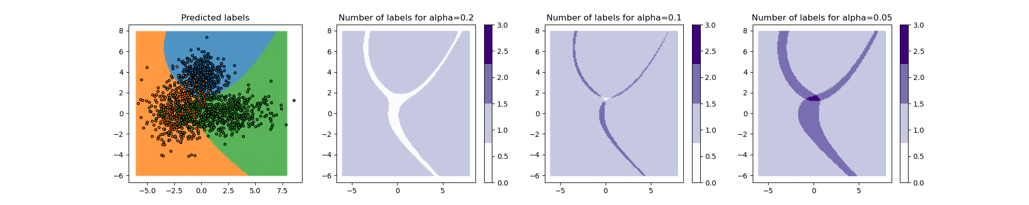
Reproducing Example 7 from Sadinle et al. (2019)

We use MapieClassifier to reproduce Example 7 from Sadinle et al. (2019).

We consider a two-dimensional dataset with three labels. The distribution of the data is a bivariate normal with diagonal covariance matrices for each label. We model the data with Gaussian Naive Bayes classifier GaussianNB as a base model.

Prediction sets are estimated by MapieClassifier from the distribution of the softmax scores of the true labels for three alpha values (0.2, 0.1, and 0.05) giving different class coverage levels.

When the class coverage level is not large enough, the prediction sets can be empty. This happens because the model is uncertain at the border between two labels. These so-called null regions disappear for larger coverage levels.

import matplotlib.pyplot as plt
import numpy as np
from sklearn.naive_bayes import GaussianNB

from mapie.classification import MapieClassifier

# Create training set from multivariate normal distribution
centers = [(0, 3.5), (-2, 0), (2, 0)]
# covs = [[[1, 0], [0, 1]], [[2, 0], [0, 2]], [[5, 0], [0, 1]]]
covs = [np.eye(2), np.eye(2) * 2, np.diag([5, 1])]
x_min, x_max, y_min, y_max, step = -6, 8, -6, 8, 0.1
n_samples = 500
n_classes = 3
alpha = [0.2, 0.1, 0.05]
np.random.seed(42)
X_train = np.vstack(
    [
        np.random.multivariate_normal(center, cov, n_samples)
        for center, cov in zip(centers, covs)
    ]
)
y_train = np.hstack([np.full(n_samples, i) for i in range(n_classes)])


# Create test from (x, y) coordinates
xx, yy = np.meshgrid(
    np.arange(x_min, x_max, step), np.arange(x_min, x_max, step)
)
X_test = np.stack([xx.ravel(), yy.ravel()], axis=1)

# Apply MapieClassifier on the dataset to get prediction sets
clf = GaussianNB().fit(X_train, y_train)
y_pred = clf.predict(X_test)
y_pred_proba = clf.predict_proba(X_test)
y_pred_proba_max = np.max(y_pred_proba, axis=1)
mapie = MapieClassifier(estimator=clf, cv="prefit", method="lac")
mapie.fit(X_train, y_train)
y_pred_mapie, y_ps_mapie = mapie.predict(X_test, alpha=alpha)

# Plot the results
tab10 = plt.cm.get_cmap("Purples", 4)
colors = {0: "#1f77b4", 1: "#ff7f0e", 2: "#2ca02c", 3: "#d62728"}
y_pred_col = list(map(colors.get, y_pred_mapie))
y_train_col = list(map(colors.get, y_train))
y_train_col = [colors[int(i)] for _, i in enumerate(y_train)]
fig, axs = plt.subplots(1, 4, figsize=(20, 4))
axs[0].scatter(
    X_test[:, 0], X_test[:, 1], color=y_pred_col, marker=".", s=10, alpha=0.4
)
axs[0].scatter(
    X_train[:, 0],
    X_train[:, 1],
    color=y_train_col,
    marker="o",
    s=10,
    edgecolor="k",
)
axs[0].set_title("Predicted labels")
for i, alpha_ in enumerate(alpha):
    y_ps_sums = y_ps_mapie[:, :, i].sum(axis=1)
    num_labels = axs[i + 1].scatter(
        X_test[:, 0],
        X_test[:, 1],
        c=y_ps_sums,
        marker=".",
        s=10,
        alpha=1,
        cmap=tab10,
        vmin=0,
        vmax=3,
    )
    cbar = plt.colorbar(num_labels, ax=axs[i + 1])
    axs[i + 1].set_title(f"Number of labels for alpha={alpha_}")
plt.show()