Tutorial for multilabel-classification¶

In this tutorial, we compare the prediction sets estimated by the RCPS and CRC methods implemented in MAPIE, for recall control purpose, on a two-dimensional toy dataset. We will also look at the Learn Then Test (LTT) procedure. It allows to create prediction sets for precision control.

Throughout this tutorial, we will answer the following questions:

How does the threshold vary according to the desired risk?
Is the chosen conformal method well calibrated (i.e. does the actual risk equal to the desired one) ?

import matplotlib.pyplot as plt
import numpy as np
from sklearn.model_selection import train_test_split
from sklearn.multioutput import MultiOutputClassifier
from sklearn.naive_bayes import GaussianNB

from mapie.multi_label_classification import MapieMultiLabelClassifier

1. Construction of the dataset¶

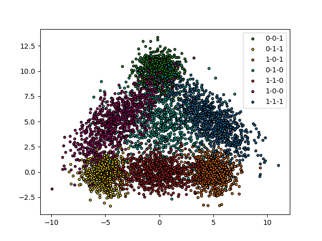
We use a two-dimensional toy dataset with three possible labels. The idea is to create a triangle where the observations on the edges have only one label, those on the vertices have two labels (those of the two edges) and the center have all the labels

centers = [(0, 10), (-5, 0), (5, 0), (0, 5), (0, 0), (-4, 5), (5, 5)]
covs = [
    np.eye(2), np.eye(2), np.eye(2), np.diag([5, 5]), np.diag([3, 1]),
    np.array([
        [4, 3],
        [3, 4]
    ]),
    np.array([
        [3, -2],
        [-2, 3]
    ]),
]

x_min, x_max, y_min, y_max, step = -15, 15, -5, 15, 0.1
n_samples = 800
X = np.vstack([
    np.random.multivariate_normal(center, cov, n_samples)
    for center, cov in zip(centers, covs)
])
classes = [
    [1, 0, 1], [1, 1, 0], [0, 1, 1], [1, 1, 1],
    [0, 1, 0], [1, 0, 0], [0, 0, 1]
]
y = np.vstack([np.full((n_samples, 3), row) for row in classes])

X_train_cal, X_test, y_train_cal, y_test = train_test_split(
    X, y, test_size=0.2
)
X_train, X_cal, y_train, y_cal = train_test_split(
    X_train_cal, y_train_cal, test_size=0.25
)

Let’s see our data.

colors = {
    (0, 0, 1): {"color": "#1f77b4", "lac": "0-0-1"},
    (0, 1, 1): {"color": "#ff7f0e", "lac": "0-1-1"},
    (1, 0, 1): {"color": "#2ca02c", "lac": "1-0-1"},
    (0, 1, 0): {"color": "#d62728", "lac": "0-1-0"},
    (1, 1, 0): {"color": "#ffd700", "lac": "1-1-0"},
    (1, 0, 0): {"color": "#c20078", "lac": "1-0-0"},
    (1, 1, 1): {"color": "#06C2AC", "lac": "1-1-1"}
}

for i in range(7):
    plt.scatter(
        X[n_samples * i:n_samples * (i + 1), 0],
        X[n_samples * i:n_samples * (i + 1), 1],
        color=colors[tuple(y[n_samples * i])]["color"],
        marker='o',
        s=10,
        edgecolor='k'
    )
plt.legend([c["lac"] for c in colors.values()])
plt.show()

2 Recall control risk with CRC and RCPS¶

2.1 Fitting MapieMultiLabelClassifier¶

MapieMultiLabelClassifier will be fitted with RCPS and CRC methods. For the RCPS method, we will test all three Upper Confidence Bounds (Hoeffding, Bernstein and Waudby-Smith–Ramdas). The two methods give two different guarantees on the risk:

RCPS: $P(R(\mathcal{T}_{\hat{\lambda}})\leq\alpha)\geq 1-\delta$

where $R(\mathcal{T}_{\hat{\lambda}})$ is the risk we want to control and $\alpha$ is the desired risk

CRC: $\mathbb{E}\left[L_{n+1}(\hat{\lambda})\right] \leq \alpha$

where $L_{n+1}(\hat{\lambda})$ is the risk of a new observation and $\alpha$ is the desired risk

In both cases, the objective of the method is to find the optimal value of $\lambda$ (threshold above which we consider a label as being present) such that the recall on the test points is at least equal to the required recall.

method_params = {
    "RCPS - Hoeffding": ("rcps", "hoeffding"),
    "RCPS - Bernstein": ("rcps", "bernstein"),
    "RCPS - WSR": ("rcps", "wsr"),
    "CRC": ("crc", None)
}

clf = MultiOutputClassifier(GaussianNB()).fit(X_train, y_train)

alpha = np.arange(0.01, 1, 0.01)
y_pss, recalls, thresholds, r_hats, r_hat_pluss = {}, {}, {}, {}, {}
y_test_repeat = np.repeat(y_test[:, :, np.newaxis], len(alpha), 2)
for i, (name, (method, bound)) in enumerate(method_params.items()):

    mapie = MapieMultiLabelClassifier(
        estimator=clf, method=method, metric_control="recall"
    )
    mapie.fit(X_cal, y_cal)

    _, y_pss[name] = mapie.predict(
        X_test, alpha=alpha, bound=bound, delta=.1
    )
    recalls[name] = (
        (y_test_repeat * y_pss[name]).sum(axis=1) /
        y_test_repeat.sum(axis=1)
    ).mean(axis=0)
    thresholds[name] = mapie.lambdas_star
    r_hats[name] = mapie.r_hat
    r_hat_pluss[name] = mapie.r_hat_plus

2.2. Results¶

To check the results of the methods, we propose two types of plots:

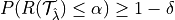
Plots where the confidence level varies. Here two metrics are plotted for each method and for each UCB
- The actual recall (which should be always near to the required one): we can see that they are close to each other.
- The value of the threshold: we see that the threshold is decreasing as $1 - \alpha$ increases, which is what is expected because a smaller threshold will give larger prediction sets, hence a larger recall.

vars_y = [recalls, thresholds]
labels_y = ["Average number of kept labels", "Recall", "Threshold"]

fig, axs = plt.subplots(1, len(vars_y), figsize=(8*len(vars_y), 8))
for i, var in enumerate(vars_y):
    for name, (method, bound) in method_params.items():
        axs[i].plot(1 - alpha, var[name], label=name, linewidth=2)
        if i == 0:
            axs[i].plot([0, 1], [0, 1], ls="--", color="k")
    axs[i].set_xlabel("Desired recall : 1 - alpha", fontsize=20)
    axs[i].set_ylabel(labels_y[i], fontsize=20)
    if i == (len(vars_y) - 1):
        axs[i].legend(fontsize=20, loc=[1, 0])
plt.show()

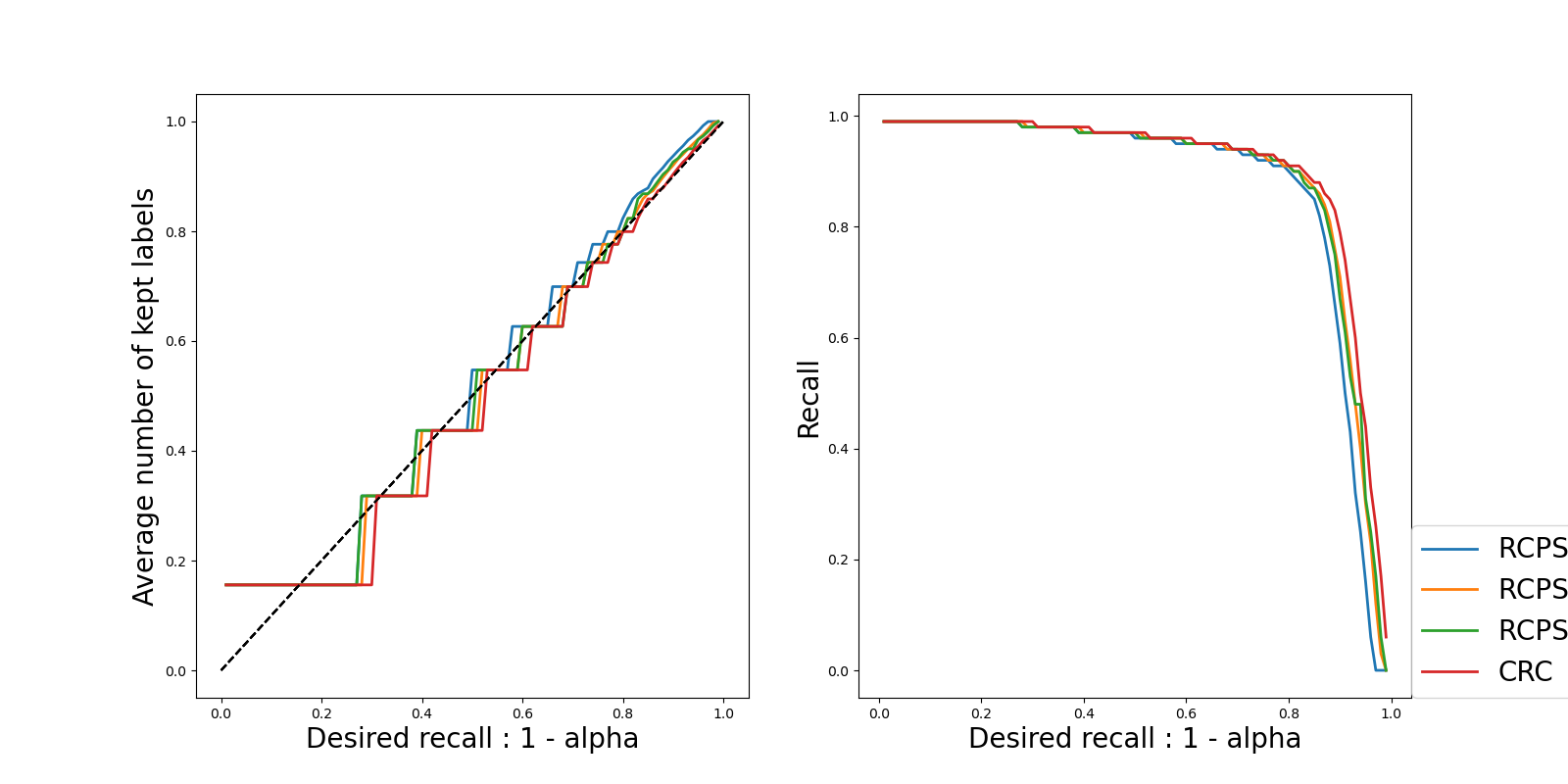
Plots where we choose a specific risk value (0.1 in our case) and look at the average risk, the UCB of the risk (for RCPS methods) and the choice of the threshold $\lambda$
- We can see that among the RCPS methods, the Bernstein method gives the best results as for a given value of $\alpha$ as we are above the required recall but with a larger value of $\lambda$ than the two others bounds.
- The CRC method gives the best results since it guarantees the coverage with a larger threshold.

fig, axs = plt.subplots(
    1,
    len(method_params),
    figsize=(8*len(method_params), 8)
)
for i, (name, (method, bound)) in enumerate(method_params.items()):
    axs[i].plot(
        mapie.lambdas,
        r_hats[name], label=r"$\hat{R}$", linewidth=2
    )
    if name != "CRC":
        axs[i].plot(
            mapie.lambdas,
            r_hat_pluss[name], label=r"$\hat{R}^+$", linewidth=2
        )
    axs[i].plot([0, 1], [alpha[9], alpha[9]], label=r"$\alpha$")
    axs[i].plot(
        [thresholds[name][9], thresholds[name][9]], [0, 1],
        label=r"$\lambda^*" + f" = {thresholds[name][9]}$"
    )
    axs[i].legend(fontsize=20)
    axs[i].set_title(
        f"{name} - Recall = {round(recalls[name][9], 2)}",
        fontsize=20
    )
plt.show()

RCPS - Hoeffding - Recall = 0.94, RCPS - Bernstein - Recall = 0.92, RCPS - WSR - Recall = 0.93, CRC - Recall = 0.9

3. Precision control risk with LTT¶

3.1 Fitting MapieMultilabelClassifier¶

In this part, we will use LTT to control precision. At the opposite of the 2 previous method, LTT can handle non-monotonous loss. The procedure consist in multiple hypothesis testing. This is why the output of this procedure isn’t reduce to one value of $\lambda$ .

More precisely, we look after all the $\lambda$ that sastisfy the following: 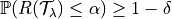$\mathbb{P}(R(\mathcal{T}_{\lambda}) \leq \alpha ) \geq 1 - \delta$ , where $R(\mathcal{T}_{\lambda})$ is the risk we want to control and each $\lambda$ should satisfy FWER control. $\alpha$ is the desired risk.

Notice that the procedure will diligently examine each $\lambda$ such that the risk remains below level $\alpha$ , meaning not every $\lambda$ will be considered. This means that a for a $\lambda$ such that risk is below $\alpha$ doesn’t necessarly pass the FWER control! This is what we are going to explore.

mapie_clf = MapieMultiLabelClassifier(
    estimator=clf,
    method='ltt',
    metric_control='precision'
)
mapie_clf.fit(X_cal, y_cal)

alpha = 0.1
_, y_ps = mapie_clf.predict(
    X_test,
    alpha=alpha,
    delta=0.1
)

valid_index = mapie_clf.valid_index[0]  # valid_index is a list of list

lambdas = mapie_clf.lambdas[valid_index]

mini = lambdas[np.argmin(lambdas)]
maxi = lambdas[np.argmax(lambdas)]

r_hat = mapie_clf.r_hat
idx_max = np.argmin(r_hat[valid_index])

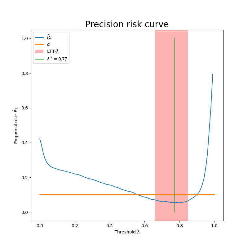
3.2 Valid parameters for precision control¶

We can see that not all $\lambda$ such that risk is below the orange line are choosen by the procedure. Otherwise, all the lambdas that are in the red rectangle verify family wise error rate control and allow to control precision at the desired level with a high probability.

plt.figure(figsize=(8, 8))
plt.plot(mapie_clf.lambdas, r_hat, label=r"$\hat{R}_\lambda$")
plt.plot([0, 1], [alpha, alpha], label=r"$\alpha$")
plt.axvspan(mini, maxi, facecolor='red', alpha=0.3, label=r"LTT-$\lambda$")
plt.plot(
    [lambdas[idx_max], lambdas[idx_max]], [0, 1],
    label=r"$\lambda^* =" + f"{lambdas[idx_max]}$"
)
plt.xlabel(r"Threshold $\lambda$")
plt.ylabel(r"Empirical risk: $\hat{R}_\lambda$")
plt.title("Precision risk curve", fontsize=20)
plt.legend()
plt.show()

Total running time of the script: ( 0 minutes 1.422 seconds)

Gallery generated by Sphinx-Gallery