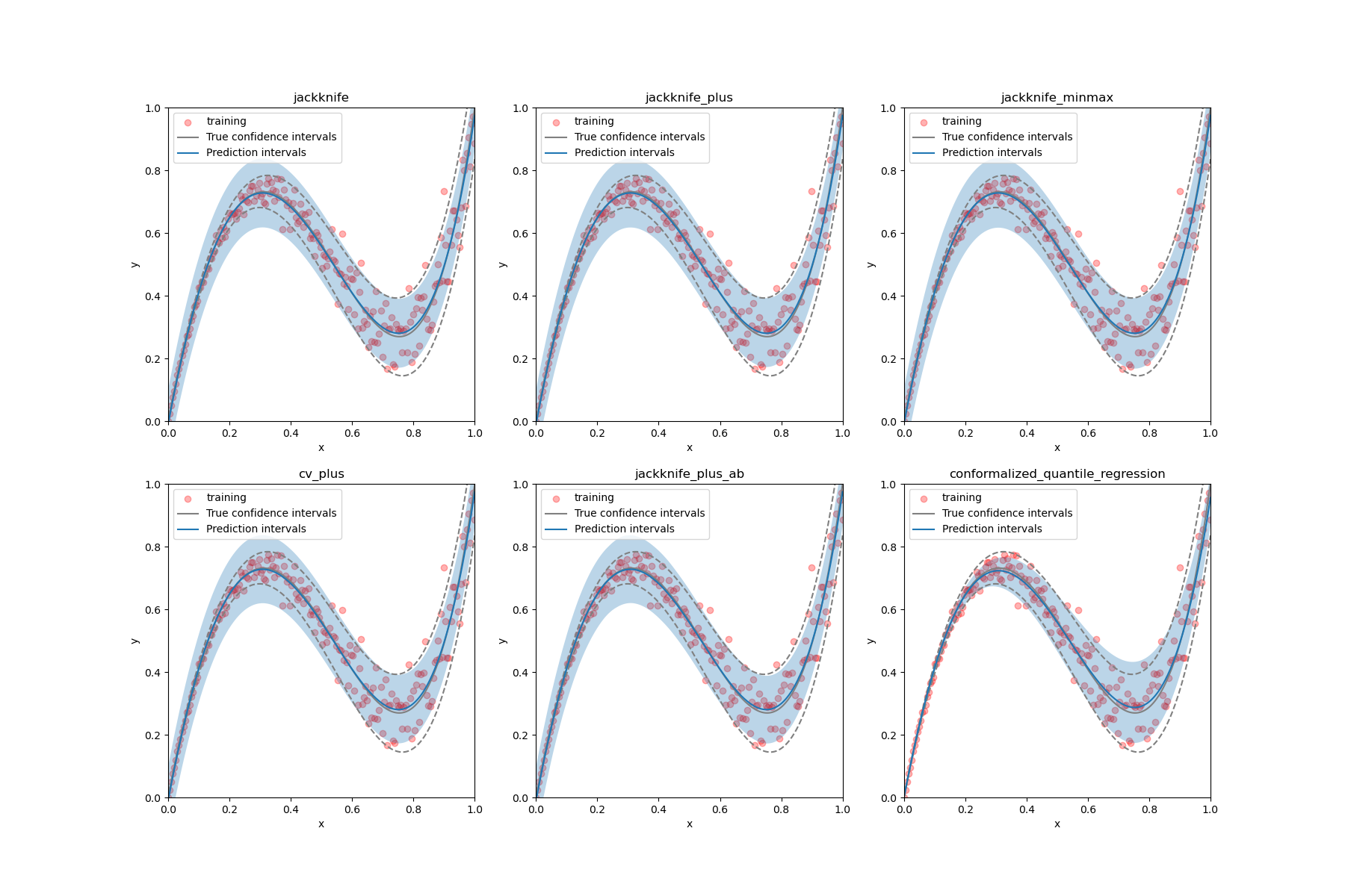
Estimate the prediction intervals of 1D heteroscedastic data

MapieRegressor and MapieQuantileRegressor is used to estimate the prediction intervals of 1D heteroscedastic data using different strategies. The latter class should provide the same coverage for a lower width of intervals because it adapts the prediction intervals to the local heteroscedastic noise.

from typing import Tuple

import numpy as np
import scipy
from matplotlib import pyplot as plt
from sklearn.linear_model import LinearRegression, QuantileRegressor
from sklearn.pipeline import Pipeline
from sklearn.preprocessing import PolynomialFeatures

from mapie._typing import NDArray
from mapie.regression import MapieQuantileRegressor, MapieRegressor
from mapie.subsample import Subsample

random_state = 42


def f(x: NDArray) -> NDArray:
    """Polynomial function used to generate one-dimensional data"""
    return np.array(5 * x + 5 * x ** 4 - 9 * x ** 2)


def get_heteroscedastic_data(
    n_train: int = 200, n_true: int = 200, sigma: float = 0.1
) -> Tuple[NDArray, NDArray, NDArray, NDArray, NDArray]:
    """
    Generate one-dimensional data from a given function,
    number of training and test samples and a given standard
    deviation increases linearly with x.
    The training data data is generated from an exponential distribution.

    Parameters
    ----------
    n_train : int, optional
        Number of training samples, by default  200.
    n_true : int, optional
        Number of test samples, by default 1000.
    sigma : float, optional
        Standard deviation of noise, by default 0.1

    Returns
    -------
    Tuple[NDArray, NDArray, NDArray, NDArray, NDArray]
        Generated training and test data.
        [0]: X_train
        [1]: y_train
        [2]: X_true
        [3]: y_true
        [4]: y_true_sigma
    """
    np.random.seed(random_state)
    q95 = scipy.stats.norm.ppf(0.95)
    X_train = np.linspace(0, 1, n_train)
    X_true = np.linspace(0, 1, n_true)
    y_train = f(X_train) + np.random.normal(0, sigma, n_train) * X_train
    y_true = f(X_true)
    y_true_sigma = q95 * sigma * X_true
    return X_train, y_train, X_true, y_true, y_true_sigma


def plot_1d_data(
    X_train: NDArray,
    y_train: NDArray,
    X_test: NDArray,
    y_test: NDArray,
    y_test_sigma: NDArray,
    y_pred: NDArray,
    y_pred_low: NDArray,
    y_pred_up: NDArray,
    ax: plt.Axes,
    title: str,
) -> None:
    """
    Generate a figure showing the training data and estimated
    prediction intervals on test data.

    Parameters
    ----------
    X_train : NDArray
        Training data.
    y_train : NDArray
        Training labels.
    X_test : NDArray
        Test data.
    y_test : NDArray
        True function values on test data.
    y_test_sigma : float
        True standard deviation.
    y_pred : NDArray
        Predictions on test data.
    y_pred_low : NDArray
        Predicted lower bounds on test data.
    y_pred_up : NDArray
        Predicted upper bounds on test data.
    ax : plt.Axes
        Axis to plot.
    title : str
        Title of the figure.
    """
    ax.set_xlabel("x")
    ax.set_ylabel("y")
    ax.set_xlim([0, 1])
    ax.set_ylim([0, 1])
    ax.scatter(X_train, y_train, color="red", alpha=0.3, label="training")
    ax.plot(X_test, y_test, color="gray", label="True confidence intervals")
    ax.plot(X_test, y_test - y_test_sigma, color="gray", ls="--")
    ax.plot(X_test, y_test + y_test_sigma, color="gray", ls="--")
    ax.plot(X_test, y_pred, label="Prediction intervals")
    ax.fill_between(X_test, y_pred_low, y_pred_up, alpha=0.3)
    ax.set_title(title)
    ax.legend()


X_train, y_train, X_test, y_test, y_test_sigma = get_heteroscedastic_data()

polyn_model = Pipeline(
    [
        ("poly", PolynomialFeatures(degree=4)),
        ("linear", LinearRegression()),
    ]
)
polyn_model_quant = Pipeline(
    [
        ("poly", PolynomialFeatures(degree=4)),
        ("linear", QuantileRegressor(
            solver="highs-ds",
            alpha=0,
        )),
    ]
)

STRATEGIES = {
    "jackknife": {"method": "base", "cv": -1},
    "jackknife_plus": {"method": "plus", "cv": -1},
    "jackknife_minmax": {"method": "minmax", "cv": -1},
    "cv_plus": {"method": "plus", "cv": 10},
    "jackknife_plus_ab": {"method": "plus", "cv": Subsample(n_resamplings=50)},
    "conformalized_quantile_regression": {"method": "quantile", "cv": "split"},
}
fig, ((ax1, ax2, ax3), (ax4, ax5, ax6)) = plt.subplots(
    2, 3, figsize=(3 * 6, 12)
)
axs = [ax1, ax2, ax3, ax4, ax5, ax6]
for i, (strategy, params) in enumerate(STRATEGIES.items()):
    if strategy == "conformalized_quantile_regression":
        mapie = MapieQuantileRegressor(  # type: ignore
            polyn_model_quant,
            **params
        )
        mapie.fit(X_train.reshape(-1, 1), y_train, random_state=random_state)
        y_pred, y_pis = mapie.predict(X_test.reshape(-1, 1))
    else:
        mapie = MapieRegressor(  # type: ignore
            polyn_model,
            agg_function="median",
            n_jobs=-1,
            **params
        )
        mapie.fit(X_train.reshape(-1, 1), y_train)
        y_pred, y_pis = mapie.predict(
            X_test.reshape(-1, 1),
            alpha=0.05,
        )
    plot_1d_data(
        X_train,
        y_train,
        X_test,
        y_test,
        y_test_sigma,
        y_pred,
        y_pis[:, 0, 0],
        y_pis[:, 1, 0],
        axs[i],
        strategy,
    )
plt.show()