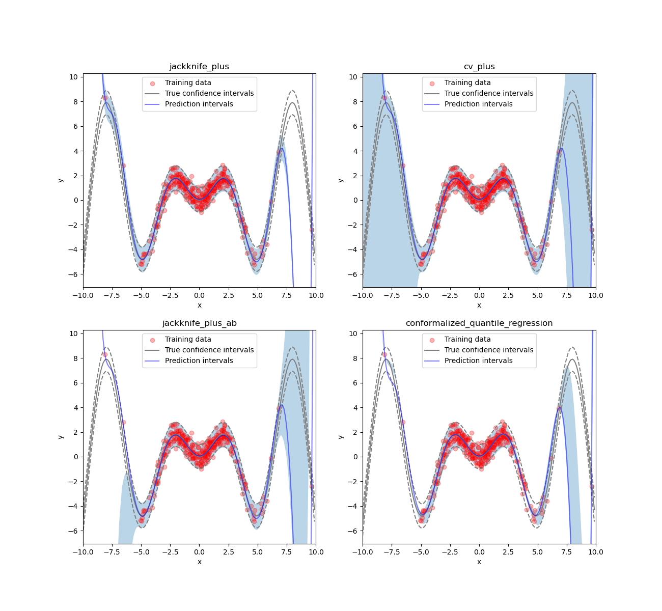
Estimating aleatoric and epistemic uncertainties

This example uses MapieRegressor and MapieQuantileRegressor to estimate prediction intervals capturing both aleatoric and epistemic uncertainties on a one-dimensional dataset with homoscedastic noise and normal sampling.

• 
• 

from typing import Any, Callable, Tuple, TypeVar

import matplotlib.pyplot as plt
import numpy as np
from sklearn.linear_model import LinearRegression, QuantileRegressor
from sklearn.pipeline import Pipeline
from sklearn.preprocessing import PolynomialFeatures

from mapie._typing import NDArray
from mapie.regression import MapieQuantileRegressor, MapieRegressor
from mapie.subsample import Subsample

F = TypeVar("F", bound=Callable[..., Any])
random_state = 42


# Functions for generating our dataset
def x_sinx(x: NDArray) -> NDArray:
    """One-dimensional x*sin(x) function."""
    return x * np.sin(x)


def get_1d_data_with_normal_distrib(
    funct: F, mu: float, sigma: float, n_samples: int, noise: float
) -> Tuple[NDArray, NDArray, NDArray, NDArray, NDArray]:
    """
    Generate noisy 1D data with normal distribution from given function
    and noise standard deviation.

    Parameters
    ----------
    funct : F
        Base function used to generate the dataset.
    mu : float
        Mean of normal training distribution.
    sigma : float
        Standard deviation of normal training distribution.
    n_samples : int
        Number of training samples.
    noise : float
        Standard deviation of noise.

    Returns
    -------
    Tuple[NDArray, AnNDArrayy, NDArray, NDArray, NDArray]
        Generated training and test data.
        [0]: X_train
        [1]: y_train
        [2]: X_test
        [3]: y_test
        [4]: y_mesh
    """
    np.random.seed(random_state)
    X_train = np.random.normal(mu, sigma, n_samples)
    X_test = np.arange(mu - 4 * sigma, mu + 4 * sigma, sigma / 20.0)
    y_train, y_mesh, y_test = funct(X_train), funct(X_test), funct(X_test)
    y_train += np.random.normal(0, noise, y_train.shape[0])
    y_test += np.random.normal(0, noise, y_test.shape[0])
    return (
        X_train.reshape(-1, 1),
        y_train,
        X_test.reshape(-1, 1),
        y_test,
        y_mesh,
    )


# Data generation
mu, sigma, n_samples, noise = 0, 2.5, 300, 0.5
X_train, y_train, X_test, y_test, y_mesh = get_1d_data_with_normal_distrib(
    x_sinx, mu, sigma, n_samples, noise
)

# Definition of our base model
degree_polyn = 10
polyn_model = Pipeline(
    [
        ("poly", PolynomialFeatures(degree=degree_polyn)),
        ("linear", LinearRegression()),
    ]
)
polyn_model_quant = Pipeline(
    [
        ("poly", PolynomialFeatures(degree=degree_polyn)),
        ("linear", QuantileRegressor(
            alpha=0,
            solver="highs",  # highs-ds does not give good results
            )),
    ]
)


# Estimating prediction intervals
STRATEGIES = {
    "jackknife_plus": {"method": "plus", "cv": -1},
    "cv_plus": {"method": "plus", "cv": 10},
    "jackknife_plus_ab": {"method": "plus", "cv": Subsample(n_resamplings=50)},
    "conformalized_quantile_regression": {"method": "quantile", "cv": "split"},
}
y_pred, y_pis = {}, {}
for strategy, params in STRATEGIES.items():
    if strategy == "conformalized_quantile_regression":
        mapie = MapieQuantileRegressor(  # type: ignore
            polyn_model_quant,
            **params
        )
        mapie.fit(X_train, y_train, random_state=random_state)
        y_pred[strategy], y_pis[strategy] = mapie.predict(X_test)
    else:
        mapie = MapieRegressor(polyn_model, **params)  # type: ignore
        mapie.fit(X_train, y_train)
        y_pred[strategy], y_pis[strategy] = mapie.predict(X_test, alpha=0.05)


# Visualization
def plot_1d_data(
    X_train: NDArray,
    y_train: NDArray,
    X_test: NDArray,
    y_test: NDArray,
    y_sigma: float,
    y_pred: NDArray,
    y_pred_low: NDArray,
    y_pred_up: NDArray,
    ax: plt.Axes,
    title: str,
) -> None:
    ax.set_xlabel("x")
    ax.set_ylabel("y")
    ax.set_xlim([-10, 10])
    ax.set_ylim([np.min(y_test) * 1.3, np.max(y_test) * 1.3])
    ax.fill_between(X_test, y_pred_low, y_pred_up, alpha=0.3)
    ax.scatter(X_train, y_train, color="red", alpha=0.3, label="Training data")
    ax.plot(X_test, y_test, color="gray", label="True confidence intervals")
    ax.plot(X_test, y_test - y_sigma, color="gray", ls="--")
    ax.plot(X_test, y_test + y_sigma, color="gray", ls="--")
    ax.plot(X_test, y_pred, color="b", alpha=0.5, label="Prediction intervals")
    if title is not None:
        ax.set_title(title)
    ax.legend()


n_figs = len(STRATEGIES)
fig, axs = plt.subplots(2, 2, figsize=(13, 12))
coords = [axs[0, 0], axs[0, 1], axs[1, 0], axs[1, 1]]
for strategy, coord in zip(STRATEGIES, coords):
    plot_1d_data(
        X_train.ravel(),
        y_train.ravel(),
        X_test.ravel(),
        y_mesh.ravel(),
        1.96 * noise,
        y_pred[strategy].ravel(),
        y_pis[strategy][:, 0, 0].ravel(),
        y_pis[strategy][:, 1, 0].ravel(),
        ax=coord,
        title=strategy,
    )


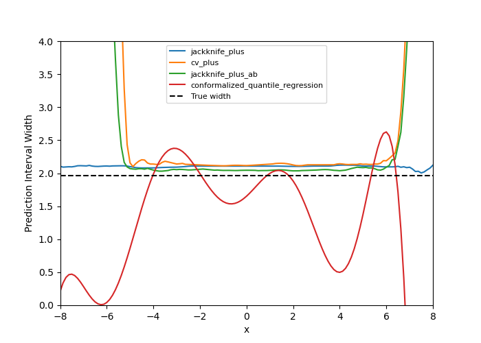
fig, ax = plt.subplots(1, 1, figsize=(7, 5))
ax.set_xlim([-8, 8])
ax.set_ylim([0, 4])
for strategy in STRATEGIES:
    ax.plot(X_test, y_pis[strategy][:, 1, 0] - y_pis[strategy][:, 0, 0])
ax.axhline(1.96 * 2 * noise, ls="--", color="k")
ax.set_xlabel("x")
ax.set_ylabel("Prediction Interval Width")
ax.legend(list(STRATEGIES.keys()) + ["True width"], fontsize=8)
plt.show()