Nested cross-validation for estimating prediction intervals

This example compares non-nested and nested cross-validation strategies for estimating prediction intervals with MapieRegressor.

In the regular sequential method, a cross-validation parameter search is carried out over the entire training set. The model with the set of parameters that gives the best score is then used in MAPIE to estimate the prediction intervals associated with the predictions. A limitation of this method is that residuals used by MAPIE are computed on the validation dataset, which can be subject to overfitting as far as hyperparameter tuning is concerned.

This fools MAPIE into being slightly too optimistic with confidence intervals. To solve this problem, an alternative option is to perform a nested cross-validation parameter search directly within the MAPIE estimator on each out-of-fold dataset. For each testing fold used by MAPIE to store residuals, an internal cross-validation occurs on the training fold, optimizing hyperparameters. This ensures that residuals seen by MAPIE are never seen by the algorithm beforehand. However, this method is much heavier computationally since it results in calculations, where N is the number of out-of-fold models and P the number of parameter search cross-validations, versus for the non-nested approach.

Here, we compare the two strategies on the Boston dataset. We use the Random Forest Regressor as a base regressor for the CV+ strategy. For the sake of light computation, we adopt a RandomizedSearchCV parameter search strategy with a low number of iterations and with a reproducible random state.

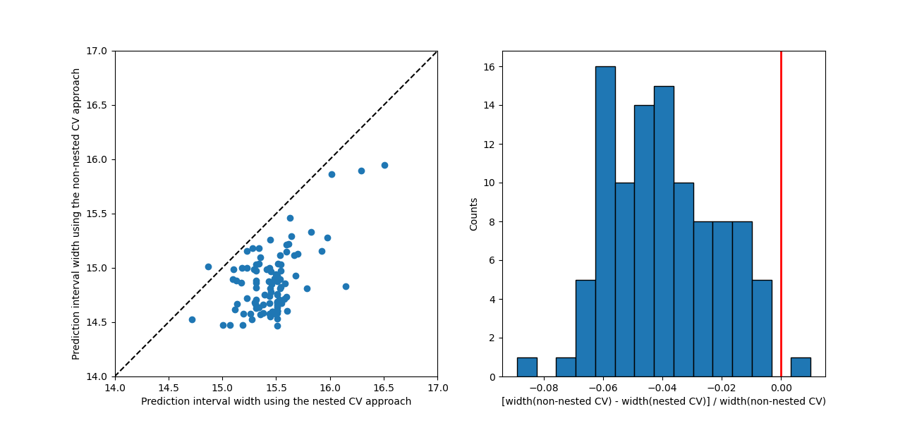
The two approaches give slightly different predictions with the nested CV approach estimating slightly larger prediction interval widths by a few percents at most (apart from a handful of exceptions).

For this example, the two approaches result in identical scores and identical effective coverages.

In the general case, the recommended approach is to use nested cross-validation, since it does not underestimate conformity scores and hence prediction intervals. However, in this particular example, effective coverages of both nested and non-nested methods are the same.

Out:

Scores and effective coverages for the CV+ strategy using the Random Forest model.
Score on the test set for the non-nested and nested CV approaches:   2.989,  2.989
Effective coverage on the test set for the non-nested and nested CV approaches:   0.980,  0.980

import matplotlib.pyplot as plt
import numpy as np
import pandas as pd
from scipy.stats import randint
from sklearn.ensemble import RandomForestRegressor
from sklearn.metrics import mean_squared_error
from sklearn.model_selection import RandomizedSearchCV, train_test_split

from mapie.metrics import regression_coverage_score
from mapie.regression import MapieRegressor

# Load the Boston data
data_url = "http://lib.stat.cmu.edu/datasets/boston"
raw_df = pd.read_csv(data_url, sep=r'\s+', skiprows=22, header=None)
X_boston = np.hstack([raw_df.values[::2, :], raw_df.values[1::2, :2]])
y_boston = raw_df.values[1::2, 2]

# Split the data into training and test sets.
X_train, X_test, y_train, y_test = train_test_split(
    X_boston, y_boston, test_size=0.2, random_state=42
)

# Define the Random Forest model as base regressor with parameter ranges.
rf_model = RandomForestRegressor(random_state=59, verbose=0)
rf_params = {"max_depth": randint(2, 10), "n_estimators": randint(10, 100)}

# Cross-validation and prediction-interval parameters.
cv = 10
n_iter = 5
alpha = 0.05
random_state = 59

# Non-nested approach with the CV+ strategy using the Random Forest model.
cv_obj = RandomizedSearchCV(
    rf_model,
    param_distributions=rf_params,
    n_iter=n_iter,
    cv=cv,
    scoring="neg_root_mean_squared_error",
    return_train_score=True,
    verbose=0,
    random_state=random_state,
    n_jobs=-1,
)
cv_obj.fit(X_train, y_train)
best_est = cv_obj.best_estimator_
mapie_non_nested = MapieRegressor(
    best_est, method="plus", cv=cv, agg_function="median", n_jobs=-1,
    random_state=random_state
)
mapie_non_nested.fit(X_train, y_train)
y_pred_non_nested, y_pis_non_nested = mapie_non_nested.predict(
    X_test, alpha=alpha
)
widths_non_nested = y_pis_non_nested[:, 1, 0] - y_pis_non_nested[:, 0, 0]
coverage_non_nested = regression_coverage_score(
    y_test, y_pis_non_nested[:, 0, 0], y_pis_non_nested[:, 1, 0]
)
score_non_nested = mean_squared_error(y_test, y_pred_non_nested, squared=False)

# Nested approach with the CV+ strategy using the Random Forest model.
cv_obj = RandomizedSearchCV(
    rf_model,
    param_distributions=rf_params,
    n_iter=n_iter,
    cv=cv,
    scoring="neg_root_mean_squared_error",
    return_train_score=True,
    verbose=0,
    random_state=random_state,
    n_jobs=-1,
)
mapie_nested = MapieRegressor(
    cv_obj, method="plus", cv=cv, agg_function="median",
    random_state=random_state
)
mapie_nested.fit(X_train, y_train)
y_pred_nested, y_pis_nested = mapie_nested.predict(X_test, alpha=alpha)
widths_nested = y_pis_nested[:, 1, 0] - y_pis_nested[:, 0, 0]
coverage_nested = regression_coverage_score(
    y_test, y_pis_nested[:, 0, 0], y_pis_nested[:, 1, 0]
)
score_nested = mean_squared_error(y_test, y_pred_nested, squared=False)

# Print scores and effective coverages.
print(
    "Scores and effective coverages for the CV+ strategy using the "
    "Random Forest model."
)
print(
    "Score on the test set for the non-nested and nested CV approaches: ",
    f"{score_non_nested: .3f}, {score_nested: .3f}",
)
print(
    "Effective coverage on the test set for the non-nested "
    "and nested CV approaches: ",
    f"{coverage_non_nested: .3f}, {coverage_nested: .3f}",
)

# Compare prediction interval widths.
fig, (ax1, ax2) = plt.subplots(1, 2, figsize=(13, 6))
min_x = 14.0
max_x = 17.0
ax1.set_xlabel("Prediction interval width using the nested CV approach")
ax1.set_ylabel("Prediction interval width using the non-nested CV approach")
ax1.set_xlim([min_x, max_x])
ax1.set_ylim([min_x, max_x])
ax1.scatter(widths_nested, widths_non_nested)
ax1.plot([min_x, max_x], [min_x, max_x], ls="--", color="k")
ax2.axvline(x=0, color="r", lw=2)
ax2.set_xlabel(
    "[width(non-nested CV) - width(nested CV)] / width(non-nested CV)"
)
ax2.set_ylabel("Counts")
ax2.hist(
    (widths_non_nested - widths_nested) / widths_non_nested,
    bins=15,
    edgecolor="black",
)
plt.show()