Quick Start with MAPIE
This package allows you to easily estimate uncertainties in both regression and classification settings. In regression settings, MAPIE provides prediction intervals on single-output data. In classification settings, MAPIE provides prediction sets on multi-class data. In any case, MAPIE is compatible with any scikit-learn-compatible estimator.
Estimate your prediction intervals
1. Download and install the module
Install via pip:
pip install mapie
or via conda:
$ conda install -c conda-forge mapie
To install directly from the github repository :
pip install git+https://github.com/scikit-learn-contrib/MAPIE
2. Run MapieRegressor
Let us start with a basic regression problem. Here, we generate one-dimensional noisy data that we fit with a linear model.
import numpy as np
from sklearn.linear_model import LinearRegression
from sklearn.datasets import make_regression
from sklearn.model_selection import train_test_split

regressor = LinearRegression()
X, y = make_regression(n_samples=500, n_features=1, noise=20, random_state=59)
X_train, X_test, y_train, y_test = train_test_split(X, y, test_size=0.5)
Since MAPIE is compliant with the standard scikit-learn API, we follow the standard
sequential fit and predict process like any scikit-learn regressor.
We set two values for alpha to estimate prediction intervals at approximately one
and two standard deviations from the mean.
from mapie.regression import MapieRegressor

mapie_regressor = MapieRegressor(regressor)
mapie_regressor.fit(X_train, y_train)

alpha = [0.05, 0.32]
y_pred, y_pis = mapie_regressor.predict(X_test, alpha=alpha)
MAPIE returns a np.ndarray of shape (n_samples, 3, len(alpha)) giving the predictions,
as well as the lower and upper bounds of the prediction intervals for the target quantile
for each desired alpha value.
You can compute the coverage of your prediction intervals.
from mapie.metrics import regression_coverage_score_v2

coverage_scores = regression_coverage_score_v2(y_test, y_pis)
The estimated prediction intervals can then be plotted as follows.
from matplotlib import pyplot as plt

plt.xlabel("x")
plt.ylabel("y")
plt.scatter(X, y, alpha=0.3)
plt.plot(X_test, y_pred, color="C1")
order = np.argsort(X_test[:, 0])
plt.plot(X_test[order], y_pis[order][:, 0, 1], color="C1", ls="--")
plt.plot(X_test[order], y_pis[order][:, 1, 1], color="C1", ls="--")
plt.fill_between(
    X_test[order].ravel(),
    y_pis[order][:, 0, 0].ravel(),
    y_pis[order][:, 1, 0].ravel(),
    alpha=0.2
)
plt.title(
    f"Target and effective coverages for "
    f"alpha={alpha[0]:.2f}: ({1-alpha[0]:.3f}, {coverage_scores[0]:.3f})\n"
    f"Target and effective coverages for "
    f"alpha={alpha[1]:.2f}: ({1-alpha[1]:.3f}, {coverage_scores[1]:.3f})"
)
plt.show()
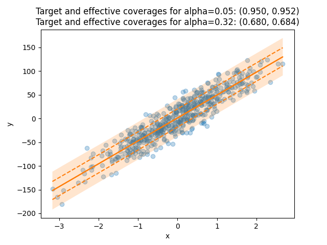
The title of the plot compares the target coverages with the effective coverages.
The target coverage, or the confidence interval, is the fraction of true labels lying in the
prediction intervals that we aim to obtain for a given dataset.
It is given by the alpha parameter defined in MapieRegressor, here equal to 0.05 and 0.32,
thus giving target coverages of 0.95 and 0.68.
The effective coverage is the actual fraction of true labels lying in the prediction intervals.
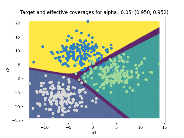
2. Run MapieClassifier
Similarly, it’s possible to do the same for a basic classification problem.
import numpy as np
from sklearn.linear_model import LogisticRegression
from sklearn.datasets import make_blobs
from sklearn.model_selection import train_test_split

classifier = LogisticRegression()
X, y = make_blobs(n_samples=500, n_features=2, centers=3)
X_train, X_test, y_train, y_test = train_test_split(X, y, test_size=0.5)
from mapie.classification import MapieClassifier

mapie_classifier = MapieClassifier(estimator=classifier, method='score', cv=5)
mapie_classifier = mapie_classifier.fit(X_train, y_train)

alpha = [0.05, 0.32]
y_pred, y_pis = mapie_classifier.predict(X_test, alpha=alpha)
from mapie.metrics import classification_coverage_score_v2

coverage_scores = classification_coverage_score_v2(y_test, y_pis)
from matplotlib import pyplot as plt

x_min, x_max = np.min(X[:, 0]), np.max(X[:, 0])
y_min, y_max = np.min(X[:, 1]), np.max(X[:, 1])
step = 0.1

xx, yy = np.meshgrid(np.arange(x_min, x_max, step), np.arange(y_min, y_max, step))
X_test_mesh = np.stack([xx.ravel(), yy.ravel()], axis=1)

y_pis = mapie_classifier.predict(X_test_mesh, alpha=alpha)[1][:,:,0]

plt.scatter(
    X_test_mesh[:, 0], X_test_mesh[:, 1],
    c=np.ravel_multi_index(y_pis.T, (2,2,2)),
    marker='.', s=10, alpha=0.2
)
plt.scatter(X[:, 0], X[:, 1], c=y, cmap='tab20c')
plt.xlabel("x1")
plt.ylabel("x2")
plt.title(
    f"Target and effective coverages for "
    f"alpha={alpha[0]:.2f}: ({1-alpha[0]:.3f}, {coverage_scores[0]:.3f})"
)
plt.show()