Theoretical Description
Three methods for multi-label uncertainty quantification have been implemented in MAPIE so far : Risk-Controlling Prediction Sets (RCPS) [1], Conformal Risk Control (CRC) [2] and Learn Then Test (LTT) [3]. The difference between these methods is the way the conformity scores are computed.
For a multi-label classification problem in a standard independent and identically distributed (i.i.d) case,
our training data  has an unknown distribution
  .
.
For any risk level  between 0 and 1, the methods implemented in MAPIE allow the user to construct a prediction
set
between 0 and 1, the methods implemented in MAPIE allow the user to construct a prediction
set  for a new observation
  with a guarantee
on the recall. RCPS, LTT, and CRC give three slightly different guarantees:
with a guarantee
on the recall. RCPS, LTT, and CRC give three slightly different guarantees:
RCPS:
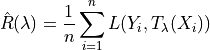
CRC:
![\mathbb{E}\left[L_{n+1}(\hat{\lambda})\right] \leq \alpha](_images/math/6bcc896c150a266188cd4463e6b87ed4d22b308a.png)
LTT:
Notice that at the opposite of the other two methods, LTT allows to control any non-monotone loss. In MAPIE for multilabel classification, we use CRC and RCPS for recall control and LTT for precision control.
1. Risk-Controlling Prediction Sets
1.1. General settings
Let’s first give the settings and the notations of the method:
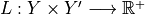
Let
 be a set-valued function (a tolerance region) that maps a feature vector to a set-valued prediction. This function is built from the model which was previously fitted on the training data. It is indexed by a one-dimensional parameter
  which is taking values in
  such that:

Let
 be a loss function on a prediction set with the following nesting property:

Let
 be the risk associated to a set-valued predictor:
![R(\mathcal{T}_{\hat{\lambda}}) = \mathbb{E}[L(Y, \mathcal{T}_{\lambda}(X))]](_images/math/a32b90487aaaaa378071172fe9f890a8143c3df7.png)
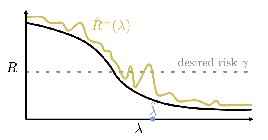
The goal of the method is to compute an Upper Confidence Bound (UCB)  of
of  and then to find
 as follows:

The figure below explains this procedure:
Following those settings, the RCPS method gives the following guarantee on the recall:
1.2. Bounds calculation
In this section, we will consider only bounded losses (as for now, only the  loss is implemented).
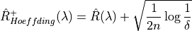
We will show three different Upper Calibration Bounds (UCB) (Hoeffding, Bernstein, and Waudby-Smith–Ramdas) of
based on the empirical risk which is defined as follows:
loss is implemented).
We will show three different Upper Calibration Bounds (UCB) (Hoeffding, Bernstein, and Waudby-Smith–Ramdas) of
based on the empirical risk which is defined as follows:
1.2.1. Hoeffding Bound
Suppose the loss is bounded above by one, then we have by the Hoeffding inequality that:

Which implies the following UCB:
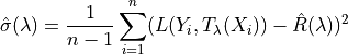
1.2.2. Bernstein Bound
Contrary to the Hoeffding bound, which can sometimes be too simple, the Bernstein UCB takes into account the variance and gives a smaller prediction set size:
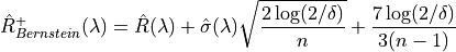
Where:
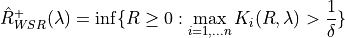
1.2.3. Waudby-Smith–Ramdas
This last UCB is the one recommended by the authors of [1] to use when using a bounded loss as this is the one that gives the smallest prediction sets size while having the same risk guarantees. This UCB is defined as follows:
Let  and
and

Further let:
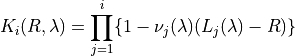
Then:
2. Conformal Risk Control
The goal of this method is to control any monotone and bounded loss. The result of this method can be expressed as follows:
Where 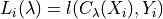
In the case of multi-label classification, 
To find the optimal value of , the following algorithm is applied:
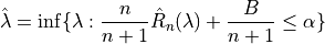
With :

3. Learn Then Test
3.1. General settings
We are going to present the Learn Then Test framework that allows the user to control non-monotonic risk such as precision score. This method has been introduced in article [3]. The settings here are the same as RCPS and CRC, we just need to introduce some new parameters:
Let
 be a discretized for our , meaning that
 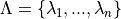 .
.Let
 be a valid p-value for the null hypothesis
  .
.
The goal of this method is to control any loss whether monotonic, bounded, or not, by performing risk control through multiple hypothesis testing. We can express the goal of the procedure as follows:
In order to find all the parameters that satisfy the above condition, the Learn Then Test framework proposes to do the following:
First across the collections of functions
 , we estimate the risk on the calibration data
 .
.For each
 in a discrete set
  , we associate the null hypothesis
 , as rejecting the hypothesis corresponds to selecting as a point where risk the risk
is controlled.
, as rejecting the hypothesis corresponds to selecting as a point where risk the risk
is controlled.For each null hypothesis, we compute a valid p-value using a concentration inequality
 . Here we choose to compute the Hoeffding-Bentkus p-value
introduced in the paper [3].
. Here we choose to compute the Hoeffding-Bentkus p-value
introduced in the paper [3].Return
 , where
  , is an algorithm
that controls the family-wise error rate (FWER), for example, Bonferonni correction.
, is an algorithm
that controls the family-wise error rate (FWER), for example, Bonferonni correction.
4. References
[1] Lihua Lei Jitendra Malik Stephen Bates, Anastasios Angelopoulos, and Michael I. Jordan. Distribution-free, risk-controlling prediction sets. CoRR, abs/2101.02703, 2021. URL https://arxiv.org/abs/2101.02703.39
[2] Angelopoulos, Anastasios N., Stephen, Bates, Adam, Fisch, Lihua, Lei, and Tal, Schuster. “Conformal Risk Control.” (2022).
[3] Angelopoulos, A. N., Bates, S., Candès, E. J., Jordan, M. I., & Lei, L. (2021). Learn then test: “Calibrating predictive algorithms to achieve risk control”.