Time series: example of the EnbPI technique

Note: in this example, we use the following terms employed in the scientific literature:

• alpha is equivalent to 1 - confidence_level. It can be seen as a risk level

• calibrate and calibration are equivalent to conformalize and conformalization.

—

This example uses TimeSeriesRegressor to estimate prediction intervals associated with time series forecast. It follows [6].

We use here the Victoria electricity demand dataset used in the book “Forecasting: Principles and Practice” by R. J. Hyndman and G. Athanasopoulos. The electricity demand features daily and weekly seasonalities and is impacted by the temperature, considered here as a exogeneous variable.

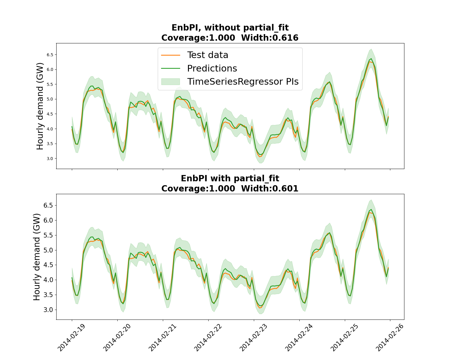
A Random Forest model is already fitted on data. The hyper-parameters are optimized with a RandomizedSearchCV using a sequential TimeSeriesSplit cross validation, in which the training set is prior to the validation set. The best model is then feeded into TimeSeriesRegressor to estimate the associated prediction intervals. We compare two approaches: with or without partial_fit called at every step following [6]. It appears that partial_fit offer a coverage closer to the targeted coverage, and with narrower PIs.

Out:

EnbPI, with no partial_fit, width optimization
WARNING:root:The option to optimize beta (minimize interval width) is not working and needs to be fixed. See more details in https://github.com/scikit-learn-contrib/MAPIE/issues/588
EnbPI with partial_fit, width optimization
WARNING:root:The option to optimize beta (minimize interval width) is not working and needs to be fixed. See more details in https://github.com/scikit-learn-contrib/MAPIE/issues/588
Coverage / prediction interval width mean for TimeSeriesRegressor:
EnbPI without any partial_fit:1.000, 0.616
Coverage / prediction interval width mean for TimeSeriesRegressor:
EnbPI with partial_fit:1.000, 0.601

import warnings
from typing import cast

import numpy as np
import pandas as pd
from matplotlib import pylab as plt
from scipy.stats import randint
from sklearn.ensemble import RandomForestRegressor
from sklearn.model_selection import RandomizedSearchCV, TimeSeriesSplit

from numpy.typing import NDArray
from mapie.metrics.regression import (
    regression_coverage_score,
    regression_mean_width_score,
)
from mapie.regression import TimeSeriesRegressor
from mapie.subsample import BlockBootstrap

warnings.simplefilter("ignore")


# Load input data and feature engineering
url_file = (
    "https://raw.githubusercontent.com/scikit-learn-contrib/MAPIE/"
    + "master/examples/data/demand_temperature.csv"
)
demand_df = pd.read_csv(url_file, parse_dates=True, index_col=0)

demand_df["Date"] = pd.to_datetime(demand_df.index)
demand_df["Weekofyear"] = demand_df.Date.dt.isocalendar().week.astype("int64")
demand_df["Weekday"] = demand_df.Date.dt.isocalendar().day.astype("int64")
demand_df["Hour"] = demand_df.index.hour
n_lags = 5
for hour in range(1, n_lags):
    demand_df[f"Lag_{hour}"] = demand_df["Demand"].shift(hour)

# Train/validation/test split
num_test_steps = 24 * 7
demand_train = demand_df.iloc[:-num_test_steps, :].copy()
demand_test = demand_df.iloc[-num_test_steps:, :].copy()
features = ["Weekofyear", "Weekday", "Hour", "Temperature"] + [
    f"Lag_{hour}" for hour in range(1, n_lags)
]

X_train = demand_train.loc[
    ~np.any(demand_train[features].isnull(), axis=1), features
]
y_train = demand_train.loc[X_train.index, "Demand"]
X_test = demand_test.loc[:, features]
y_test = demand_test["Demand"]

perform_hyperparameters_search = False
if perform_hyperparameters_search:
    # CV parameter search
    n_iter = 100
    n_splits = 5
    tscv = TimeSeriesSplit(n_splits=n_splits)
    random_state = 59
    rf_model = RandomForestRegressor(random_state=random_state)
    rf_params = {"max_depth": randint(2, 30), "n_estimators": randint(10, 100)}
    cv_obj = RandomizedSearchCV(
        rf_model,
        param_distributions=rf_params,
        n_iter=n_iter,
        cv=tscv,
        scoring="neg_root_mean_squared_error",
        random_state=random_state,
        verbose=0,
        n_jobs=-1,
    )
    cv_obj.fit(X_train, y_train)
    model = cv_obj.best_estimator_
else:
    # Model: Random Forest previously optimized with a cross-validation
    model = RandomForestRegressor(
        max_depth=10, n_estimators=50, random_state=59
    )

# Estimate prediction intervals on test set with best estimator
alpha = 0.05
cv_mapietimeseries = BlockBootstrap(
    n_resamplings=10, n_blocks=10, overlapping=False, random_state=59
)

mapie_enpbi = TimeSeriesRegressor(
    model,
    method="enbpi",
    cv=cv_mapietimeseries,
    agg_function="mean",
    n_jobs=-1,
)

print("EnbPI, with no partial_fit, width optimization")
mapie_enpbi = mapie_enpbi.fit(X_train, y_train)
y_pred_npfit_enbpi, y_pis_npfit_enbpi = mapie_enpbi.predict(
    X_test, confidence_level=1-alpha, ensemble=True, optimize_beta=True
)
coverage_npfit_enbpi = regression_coverage_score(
    y_test, y_pis_npfit_enbpi
)[0]

width_npfit_enbpi = regression_mean_width_score(
    y_pis_npfit_enbpi
)[0]

print("EnbPI with partial_fit, width optimization")
mapie_enpbi = mapie_enpbi.fit(X_train, y_train)
y_pred_pfit_enbpi = np.zeros(y_pred_npfit_enbpi.shape)
y_pis_pfit_enbpi = np.zeros(y_pis_npfit_enbpi.shape)

step_size = 1
(
    y_pred_pfit_enbpi[:step_size],
    y_pis_pfit_enbpi[:step_size, :, :],
) = mapie_enpbi.predict(
    X_test.iloc[:step_size, :], confidence_level=1-alpha, ensemble=True,
    optimize_beta=True
)

for step in range(step_size, len(X_test), step_size):
    mapie_enpbi.partial_fit(
        X_test.iloc[(step - step_size):step, :],
        y_test.iloc[(step - step_size):step],
    )
    (
        y_pred_pfit_enbpi[step:step + step_size],
        y_pis_pfit_enbpi[step:step + step_size, :, :],
    ) = mapie_enpbi.predict(
        X_test.iloc[step:(step + step_size), :],
        confidence_level=1-alpha,
        ensemble=True,
    )
coverage_pfit_enbpi = regression_coverage_score(
    y_test, y_pis_pfit_enbpi
)[0]
width_pfit_enbpi = regression_mean_width_score(
    y_pis_pfit_enbpi
)[0]

# Print results
print(
    "Coverage / prediction interval width mean for TimeSeriesRegressor: "
    "\nEnbPI without any partial_fit:"
    f"{coverage_npfit_enbpi:.3f}, {width_npfit_enbpi:.3f}"
)
print(
    "Coverage / prediction interval width mean for TimeSeriesRegressor: "
    "\nEnbPI with partial_fit:"
    f"{coverage_pfit_enbpi:.3f}, {width_pfit_enbpi:.3f}"
)

enbpi_no_pfit = {
    "y_pred": y_pred_npfit_enbpi,
    "y_pis": y_pis_npfit_enbpi,
    "coverage": coverage_npfit_enbpi,
    "width": width_npfit_enbpi,
}

enbpi_pfit = {
    "y_pred": y_pred_pfit_enbpi,
    "y_pis": y_pis_pfit_enbpi,
    "coverage": coverage_pfit_enbpi,
    "width": width_pfit_enbpi,
}

results = [enbpi_no_pfit, enbpi_pfit]

# Plot estimated prediction intervals on test set
fig, axs = plt.subplots(
    nrows=2, ncols=1, figsize=(15, 12), sharex="col"
)

for i, (ax, w, result) in enumerate(
    zip(axs, ["EnbPI, without partial_fit", "EnbPI with partial_fit"], results)
):
    ax.set_ylabel("Hourly demand (GW)", fontsize=20)
    ax.plot(demand_test.Demand, lw=2, label="Test data", c="C1")

    ax.plot(
        demand_test.index,
        result["y_pred"],
        lw=2,
        c="C2",
        label="Predictions",
    )

    y_pis = cast(NDArray, result["y_pis"])

    ax.fill_between(
        demand_test.index,
        y_pis[:, 0, 0],
        y_pis[:, 1, 0],
        color="C2",
        alpha=0.2,
        label="TimeSeriesRegressor PIs",
    )

    ax.set_title(
        w + "\n"
        f"Coverage:{result['coverage']:.3f}  Width:{result['width']:.3f}",
        fontweight="bold",
        size=20
    )
    plt.xticks(size=15, rotation=45)
    plt.yticks(size=15)

axs[0].legend(prop={'size': 22})
plt.show()