Use MAPIE to control the precision of a binary classifier

In this example, we explain how to do risk control for binary classification with MAPIE.

import numpy as np
import matplotlib.pyplot as plt
from sklearn.datasets import make_circles
from sklearn.svm import SVC
from sklearn.model_selection import FixedThresholdClassifier
from sklearn.metrics import precision_score
from sklearn.inspection import DecisionBoundaryDisplay

from mapie.risk_control import BinaryClassificationController, precision
from mapie.utils import train_conformalize_test_split

RANDOM_STATE = 1

Let us first load the dataset and fit an SVC on the training data.

X, y = make_circles(n_samples=3000, noise=0.3, factor=0.3, random_state=RANDOM_STATE)
(X_train, X_calib, X_test,
 y_train, y_calib, y_test) = train_conformalize_test_split(
     X, y,
     train_size=0.8, conformalize_size=0.1, test_size=0.1,
     random_state=RANDOM_STATE
     )

clf = SVC(probability=True, random_state=RANDOM_STATE)
clf.fit(X_train, y_train)

SVC(probability=True, random_state=1)

In a Jupyter environment, please rerun this cell to show the HTML representation or trust the notebook.
On GitHub, the HTML representation is unable to render, please try loading this page with nbviewer.org.

Next, we initialize a BinaryClassificationController using the probability estimation function from the fitted estimator: clf.predict_proba, a risk function (here the precision), a target risk level, and a confidence level. Then we use the calibration data to compute statistically guaranteed thresholds using a risk control method.

target_precision = 0.8
confidence_level = 0.9
bcc = BinaryClassificationController(
    clf.predict_proba,
    precision, target_level=target_precision,
    confidence_level=confidence_level
    )
bcc.calibrate(X_calib, y_calib)

print(f'{len(bcc.valid_predict_params)} thresholds found that guarantee a precision of '
      f'at least {target_precision} with a confidence of {confidence_level}.\n'
      'Among those, the one that maximizes the secondary objective (recall here) is: '
      f'{bcc.best_predict_param:.3f}.')

Out:

36 thresholds found that guarantee a precision of at least 0.8 with a confidence of 0.9.
Among those, the one that maximizes the secondary objective (recall here) is: 0.590.

In the plot below, we visualize how the threshold values impact precision, and what thresholds have been computed as statistically guaranteed.

proba_positive_class = clf.predict_proba(X_calib)[:, 1]

tested_thresholds = bcc._predict_params
precisions = np.full(len(tested_thresholds), np.inf)
for i, threshold in enumerate(tested_thresholds):
    y_pred = (proba_positive_class >= threshold).astype(int)
    precisions[i] = precision_score(y_calib, y_pred)

valid_thresholds_indices = np.array(
    [t in bcc.valid_predict_params for t in tested_thresholds])
best_threshold_index = np.where(
    tested_thresholds == bcc.best_predict_param)[0][0]

plt.figure()
plt.scatter(
    tested_thresholds[valid_thresholds_indices], precisions[valid_thresholds_indices],
    c='tab:green', label='Valid thresholds'
    )
plt.scatter(
    tested_thresholds[~valid_thresholds_indices], precisions[~valid_thresholds_indices],
    c='tab:red', label='Invalid thresholds'
    )
plt.scatter(
    tested_thresholds[best_threshold_index], precisions[best_threshold_index],
    c='tab:green', label='Best threshold', marker='*', edgecolors='k', s=300
    )
plt.axhline(target_precision, color='tab:gray', linestyle='--')
plt.text(
    0.7, target_precision+0.02, 'Target precision', color='tab:gray', fontstyle='italic'
)
plt.xlabel('Threshold')
plt.ylabel('Precision')
plt.legend()
plt.show()

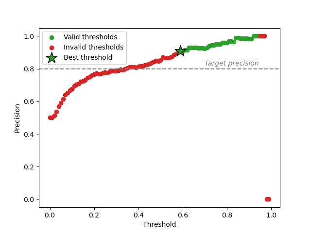
Contrary to the naive way of computing a threshold to satisfy a precision target on calibration data, risk control provides statistical guarantees on unseen data. In the plot above, we can see that not all thresholds corresponding to a precision higher that the target are valid. This is due to the uncertainty inherent to the finite size of the calibration set, which risk control takes into account.

In particular, the highest threshold values are considered invalid due to the small number of observations used to compute the precision, following the Learn then Test procedure. In the most extreme case, no observation is available, which causes the precision value to be ill-defined and set to 0.

# Besides computing a set of valid thresholds,
# :class:`~mapie.risk_control.BinaryClassificationController` also outputs the "best"
# one, which is the valid threshold that maximizes a secondary objective
# (recall here).
#
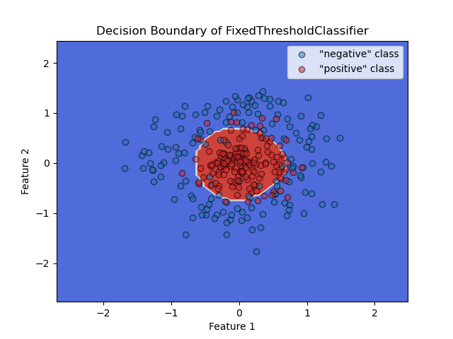
# After obtaining the best threshold, we can use the ``predict`` function of
# :class:`~mapie.risk_control.BinaryClassificationController` for future predictions,
# or use scikit-learn's ``FixedThresholdClassifier`` as a wrapper to benefit
# from functionalities like easily plotting the decision boundary as seen below.

y_pred = bcc.predict(X_test)

clf_threshold = FixedThresholdClassifier(clf, threshold=bcc.best_predict_param)
clf_threshold.fit(X_train, y_train)
# .fit necessary for plotting, alternatively you can use sklearn.frozen.FrozenEstimator


disp = DecisionBoundaryDisplay.from_estimator(
    clf_threshold, X_test, response_method="predict", cmap=plt.cm.coolwarm
    )

plt.scatter(
    X_test[y_test == 0, 0], X_test[y_test == 0, 1],
    edgecolors='k', c='tab:blue', alpha=0.5, label='"negative" class'
    )
plt.scatter(
    X_test[y_test == 1, 0], X_test[y_test == 1, 1],
    edgecolors='k', c='tab:red', alpha=0.5, label='"positive" class'
    )
plt.title("Decision Boundary of FixedThresholdClassifier")
plt.xlabel("Feature 1")
plt.ylabel("Feature 2")
plt.legend()
plt.show()

Different risk functions have been implemented, such as precision and recall, but you can also implement your own custom function using BinaryClassificationRisk and choose your own secondary objective.