Use MAPIE to control risk of a binary classifier with multiple prediction parameters

AI is a powerful tool for email sorting (for example between spam and urgent emails). However, because algorithms are not perfect, manual verification is sometimes required. Thus one would like to be able to control the amount of emails sent to human validation. One way to do so is to define a multi-parameter prediction function based on a classifier’s predicted scores. This would allow defining a rule for email checking, which could be adapted by varying the prediction parameters.

In this example, we explain how to do risk control for binary classification relying on multiple prediction parameters with MAPIE.

import matplotlib.pyplot as plt
import numpy as np
from sklearn.datasets import make_circles
from sklearn.neural_network import MLPClassifier

from mapie.risk_control import BinaryClassificationController, BinaryClassificationRisk
from mapie.utils import train_conformalize_test_split

RANDOM_STATE = 1

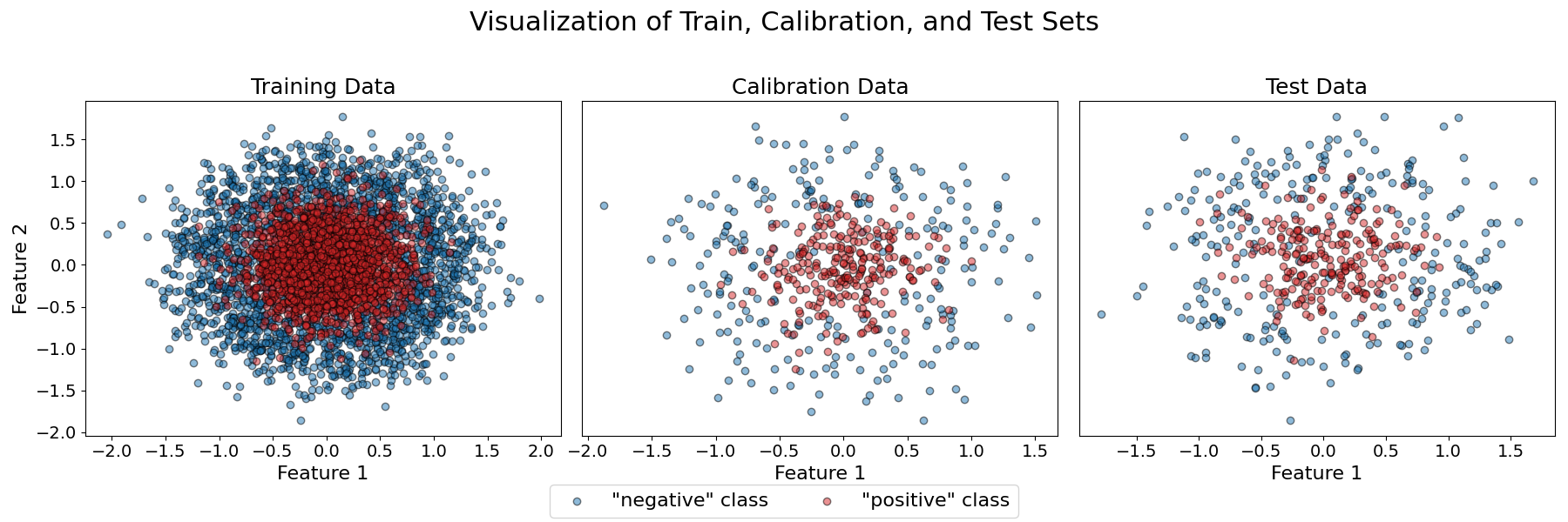
First, load the dataset and then split it into training, calibration, and test sets.

X, y = make_circles(n_samples=5000, noise=0.3, factor=0.3, random_state=RANDOM_STATE)
(X_train, X_calib, X_test, y_train, y_calib, y_test) = train_conformalize_test_split(
    X,
    y,
    train_size=0.8,
    conformalize_size=0.1,
    test_size=0.1,
    random_state=RANDOM_STATE,
)

# Plot the three datasets to visualize the distribution of the two classes. We can
# assume that the feature space represents some embedding of emails.
fig, axes = plt.subplots(1, 3, figsize=(18, 6))
titles = ["Training Data", "Calibration Data", "Test Data"]
datasets = [(X_train, y_train), (X_calib, y_calib), (X_test, y_test)]

for i, (ax, (X_data, y_data), title) in enumerate(zip(axes, datasets, titles)):
    ax.scatter(
        X_data[y_data == 0, 0],
        X_data[y_data == 0, 1],
        edgecolors="k",
        c="tab:blue",
        label='"negative" class',
        alpha=0.5,
    )
    ax.scatter(
        X_data[y_data == 1, 0],
        X_data[y_data == 1, 1],
        edgecolors="k",
        c="tab:red",
        label='"positive" class',
        alpha=0.5,
    )
    ax.set_title(title, fontsize=18)
    ax.set_xlabel("Feature 1", fontsize=16)
    ax.tick_params(labelsize=14)

    if i == 0:
        ax.set_ylabel("Feature 2", fontsize=16)
    else:
        ax.set_ylabel("")
        ax.set_yticks([])

handles, labels = axes[0].get_legend_handles_labels()
fig.legend(
    handles,
    labels,
    loc="lower center",
    bbox_to_anchor=(0.5, -0.01),
    ncol=2,
    fontsize=16,
)

plt.suptitle("Visualization of Train, Calibration, and Test Sets", fontsize=22)
plt.tight_layout(rect=[0, 0.05, 1, 0.95])
plt.show()

Second, fit a Multi-layer Perceptron classifier on the training data.

clf = MLPClassifier(max_iter=150, random_state=RANDOM_STATE)
clf.fit(X_train, y_train)

MLPClassifier(max_iter=150, random_state=1)

In a Jupyter environment, please rerun this cell to show the HTML representation or trust the notebook.
On GitHub, the HTML representation is unable to render, please try loading this page with nbviewer.org.

Third define a multi-parameter prediction function. For an email to be sent to human verification, we want the predicted score of the positive class to be between two thresholds lambda_1 and lambda_2. High (respectively low) values of the score correspond to high confidence that the email is a spam (respectively not a spam). Therefore, emails with intermediate scores are the ones for which the classifier is the least certain, and we want these emails to be verified by a human.

def send_to_human(X, lambda_1, lambda_2):
    y_score = clf.predict_proba(X)[:, 1]
    return (lambda_1 <= y_score) & (y_score < lambda_2)

From the previous function, we know we have a constraint lambda_1 <= lambda_2. We can generate a set of values to explore respecting this constraint.

to_explore = []
for i in range(6):
    lambda_1 = (i + 1) / 10
    for j in [1, 2, 3, 4, 5]:
        lambda_2 = lambda_1 + j / 10
        if lambda_2 > 0.99:
            break
        to_explore.append((lambda_1, lambda_2))
to_explore = np.array(to_explore)

Because we want to control the proportion of emails to be verified by a human, we need to define a specific BinaryClassificationRisk which represents the fraction of samples predicted as positive (i.e., sent to human verification).

prop_positive = BinaryClassificationRisk(
    risk_occurrence=lambda y_true, y_pred: y_pred,
    risk_condition=lambda y_true, y_pred: True,
    higher_is_better=False,
)

Finally, we initialize a BinaryClassificationController using our custom function send_to_human, our custom risk prop_positive, a target risk level (0.2), and a confidence level (0.9). Then we use the calibration data to compute statistically guaranteed thresholds using a multi-parameter control method.

target_level = 0.2
confidence_level = 0.9

bcc = BinaryClassificationController(
    predict_function=send_to_human,
    risk=prop_positive,
    target_level=target_level,
    confidence_level=confidence_level,
    best_predict_param_choice="precision",
    list_predict_params=to_explore,
)
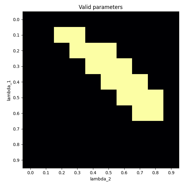
bcc.calibrate(X_calib, y_calib)

print(
    f"{len(bcc.valid_predict_params)} multi-dimensional parameters "
    f"found that guarantee a proportion of emails sent to verification\n"
    f"of at most {target_level} with a confidence of {confidence_level}."
)

16 multi-dimensional parameters found that guarantee a proportion of emails sent to verification
of at most 0.2 with a confidence of 0.9.

matrix = np.zeros((10, 10))
for valid_params in bcc.valid_predict_params:
    row = valid_params[0] * 10
    col = valid_params[1] * 10
    matrix[int(row), int(col)] = 1

fig, ax = plt.subplots(figsize=(6, 6))
im = ax.imshow(matrix, cmap="inferno")
ax.set_xticks(range(10), labels=(np.array(range(10)) / 10))
ax.set_yticks(range(10), labels=(np.array(range(10)) / 10))
ax.set_xlabel(r"lambda_2")
ax.set_ylabel(r"lambda_1")
ax.set_title("Valid parameters")
fig.tight_layout()
plt.show()