Cross-conformal for classification

In this tutorial, we estimate the impact of the training/calibration split on the prediction sets and on the resulting coverage estimated by MapieClassifier. We then adopt a cross-validation approach in which the conformity scores of all calibration sets are used to estimate the quantile. We demonstrate that this second “cross-conformal” approach gives more robust prediction sets with accurate calibration plots.

The two-dimensional dataset used here is the one presented by Sadinle et al. (2019) also introduced by other examples of this documentation.

We start the tutorial by splitting our training dataset in folds and sequentially use each fold as a calibration set, the folds remaining folds are used for training the base model using the cv="prefit" option of MapieClassifier.

from typing import Any, Dict, List, Optional, Union

import matplotlib.pyplot as plt
import numpy as np
import pandas as pd
from sklearn.model_selection import KFold
from sklearn.naive_bayes import GaussianNB
from typing_extensions import TypedDict

from mapie._typing import NDArray
from mapie.classification import MapieClassifier
from mapie.metrics import (classification_coverage_score,
                           classification_mean_width_score)

1. Estimating the impact of train/calibration split on the prediction sets

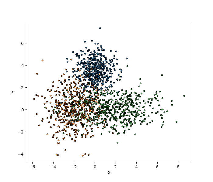
We start by generating the two-dimensional dataset and extracting training and test sets. Two test sets are created, one with the same distribution as the training set and a second one with a regular mesh for visualization. The dataset is two-dimensional with three classes, data points of each class are obtained from a normal distribution.

centers = [(0, 3.5), (-2, 0), (2, 0)]
covs = [[[1, 0], [0, 1]], [[2, 0], [0, 2]], [[5, 0], [0, 1]]]
x_min, x_max, y_min, y_max, step = -5, 7, -5, 7, 0.1
n_samples = 500
n_classes = 3
n_cv = 5
np.random.seed(42)

X_train = np.vstack([
    np.random.multivariate_normal(center, cov, n_samples)
    for center, cov in zip(centers, covs)
])
y_train = np.hstack([np.full(n_samples, i) for i in range(n_classes)])

X_test_distrib = np.vstack([
    np.random.multivariate_normal(center, cov, 10*n_samples)
    for center, cov in zip(centers, covs)
])
y_test_distrib = np.hstack(
    [np.full(10*n_samples, i) for i in range(n_classes)]
)

xx, yy = np.meshgrid(
    np.arange(x_min, x_max, step), np.arange(x_min, x_max, step)
)
X_test = np.stack([xx.ravel(), yy.ravel()], axis=1)

Let’s visualize the two-dimensional dataset.

colors = {0: "#1f77b4", 1: "#ff7f0e", 2: "#2ca02c", 3: "#d62728"}
y_train_col = list(map(colors.get, y_train))
fig = plt.figure(figsize=(7, 6))
plt.scatter(
    X_train[:, 0],
    X_train[:, 1],
    color=y_train_col,
    marker="o",
    s=10,
    edgecolor="k",
)
plt.xlabel("X")
plt.ylabel("Y")
plt.show()

We split our training dataset into 5 folds and use each fold as a calibration set. Each calibration set is therefore used to estimate the conformity scores and the given quantiles for the two methods implemented in MapieClassifier.

kf = KFold(n_splits=5, shuffle=True)
clfs, mapies, y_preds, y_ps_mapies = {}, {}, {}, {}
methods = ["lac", "aps"]
alpha = np.arange(0.01, 1, 0.01)
for method in methods:
    clfs_, mapies_, y_preds_, y_ps_mapies_ = {}, {}, {}, {}
    for fold, (train_index, calib_index) in enumerate(kf.split(X_train)):
        clf = GaussianNB().fit(X_train[train_index], y_train[train_index])
        clfs_[fold] = clf
        mapie = MapieClassifier(estimator=clf, cv="prefit", method=method)
        mapie.fit(X_train[calib_index], y_train[calib_index])
        mapies_[fold] = mapie
        y_pred_mapie, y_ps_mapie = mapie.predict(
            X_test_distrib, alpha=alpha, include_last_label="randomized"
        )
        y_preds_[fold], y_ps_mapies_[fold] = y_pred_mapie, y_ps_mapie
    clfs[method], mapies[method], y_preds[method], y_ps_mapies[method] = (
        clfs_, mapies_, y_preds_, y_ps_mapies_
    )

Let’s now plot the distribution of conformity scores for each calibration set and the estimated quantile for alpha = 0.1.

fig, axs = plt.subplots(1, len(mapies["lac"]), figsize=(20, 4))
for i, (key, mapie) in enumerate(mapies["lac"].items()):
    axs[i].set_xlabel("Conformity scores")
    axs[i].hist(mapie.conformity_scores_)
    axs[i].axvline(mapie.quantiles_[9], ls="--", color="k")
    axs[i].set_title(f"split={key}\nquantile={mapie.quantiles_[9]:.3f}")
plt.suptitle(
    "Distribution of scores on each calibration fold for the "
    f"{methods[0]} method"
)
plt.show()

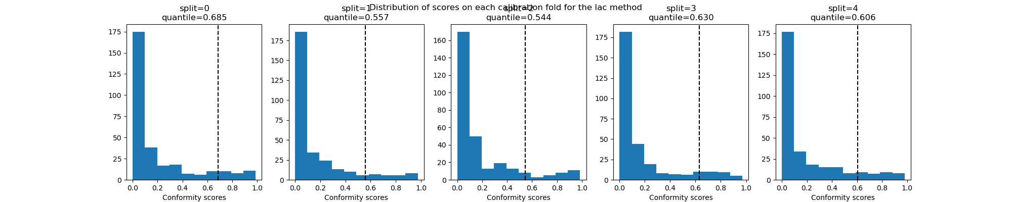
We notice that the estimated quantile slightly varies among the calibration sets for the two methods explored here, suggesting that the train/calibration splitting can slightly impact our results.

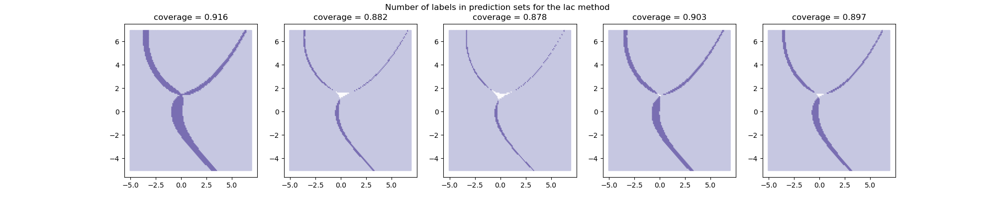
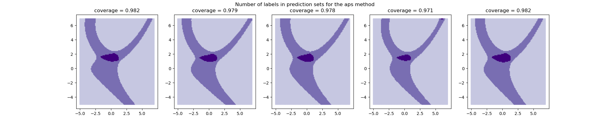
Let’s now visualize this impact on the number of labels included in each prediction set induced by the different calibration sets.

def plot_results(
    mapies: Dict[int, Any],
    X_test: NDArray,
    X_test2: NDArray,
    y_test2: NDArray,
    alpha: float,
    method: str
) -> None:
    tab10 = plt.cm.get_cmap('Purples', 4)
    fig, axs = plt.subplots(1, len(mapies), figsize=(20, 4))
    for i, (_, mapie) in enumerate(mapies.items()):
        y_pi_sums = mapie.predict(
            X_test,
            alpha=alpha,
            include_last_label=True
        )[1][:, :, 0].sum(axis=1)
        axs[i].scatter(
            X_test[:, 0],
            X_test[:, 1],
            c=y_pi_sums,
            marker='.',
            s=10,
            alpha=1,
            cmap=tab10,
            vmin=0,
            vmax=3
        )
        coverage = classification_coverage_score(
            y_test2, mapie.predict(X_test2, alpha=alpha)[1][:, :, 0]
        )
        axs[i].set_title(f"coverage = {coverage:.3f}")
    plt.suptitle(
        "Number of labels in prediction sets "
        f"for the {method} method"
    )
    plt.show()

The prediction sets and the resulting coverages slightly vary among calibration sets. Let’s now visualize the coverage score and the prediction set size as function of the alpha parameter.

plot_results(
    mapies["lac"],
    X_test,
    X_test_distrib,
    y_test_distrib,
    alpha[9],
    "lac"
)

plot_results(
    mapies["aps"],
    X_test,
    X_test_distrib,
    y_test_distrib,
    alpha[9],
    "aps"
)

• 
• 

Let’s now compare the coverages and prediction set sizes obtained with the different folds used as calibration sets.

def plot_coverage_width(
    alpha: NDArray,
    coverages: List[NDArray],
    widths: List[NDArray],
    method: str,
    comp: str = "split"
) -> None:
    if comp == "split":
        legends = [f"Split {i + 1}" for i, _ in enumerate(coverages)]
    else:
        legends = ["Mean", "Crossval"]
    _, axes = plt.subplots(nrows=1, ncols=2, figsize=(12, 5))
    axes[0].set_xlabel("1 - alpha")
    axes[0].set_ylabel("Effective coverage")
    for i, coverage in enumerate(coverages):
        axes[0].plot(1 - alpha, coverage, label=legends[i])
    axes[0].plot([0, 1], [0, 1], ls="--", color="k")
    axes[0].legend()
    axes[1].set_xlabel("1 - alpha")
    axes[1].set_ylabel("Average of prediction set sizes")
    for i, width in enumerate(widths):
        axes[1].plot(1 - alpha, width, label=legends[i])
    axes[1].legend()
    plt.suptitle(
        "Effective coverage and prediction set size "
        f"for the {method} method"
    )
    plt.show()


split_coverages = np.array(
    [
        [
            [
                classification_coverage_score(
                    y_test_distrib, y_ps[:, :, ia]
                ) for ia, _ in enumerate(alpha)]
            for _, y_ps in y_ps2.items()
        ] for _, y_ps2 in y_ps_mapies.items()
    ]
)

split_widths = np.array(
    [
        [
            [
                classification_mean_width_score(y_ps[:, :, ia])
                for ia, _ in enumerate(alpha)
            ]
            for _, y_ps in y_ps2.items()
        ] for _, y_ps2 in y_ps_mapies.items()
    ]
)

plot_coverage_width(
    alpha, split_coverages[0], split_widths[0], "lac"
)

plot_coverage_width(
    alpha, split_coverages[1], split_widths[1], "aps"
)

• 
• 

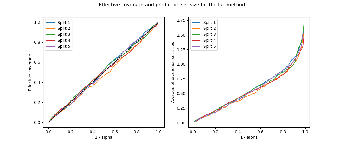
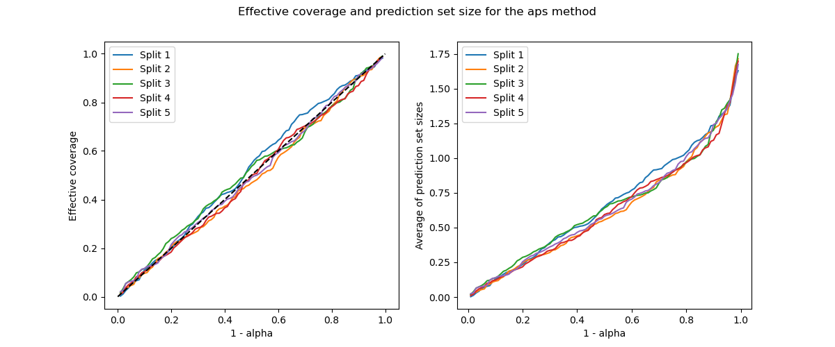
One can notice that the train/calibration indeed impacts the coverage and prediction set.

In conclusion, the split-conformal method has two main limitations:

• It prevents us to use the whole training set for training our base model

• The prediction sets are impacted by the way we extract the calibration set

2. Aggregating the conformity scores through cross-validation

It is possible to “aggregate” the predictions through cross-validation mainly via two methods:

1. Aggregating the conformity scores for all training points and then simply averaging the scores output by the different perturbed models for a new test point

2. Comparing individually the conformity scores of the training points with the conformity scores from the associated model for a new test point (as presented in Romano et al. 2020 for the “aps” method)

Let’s explore the two possibilites with the “lac” method using MapieClassifier.

All we need to do is to provide with the cv argument a cross-validation object or an integer giving the number of folds. When estimating the prediction sets, we define how the scores are aggregated with the agg_scores attribute.

Params = TypedDict(
    "Params",
    {
        "method": str,
        "cv": Optional[Union[int, str]],
        "random_state": Optional[int]
    }
)
ParamsPredict = TypedDict(
    "ParamsPredict",
    {
        "include_last_label": Union[bool, str],
        "agg_scores": str
    }
)

kf = KFold(n_splits=5, shuffle=True)

STRATEGIES = {
    "score_cv_mean": (
        Params(method="lac", cv=kf, random_state=42),
        ParamsPredict(include_last_label=False, agg_scores="mean")
    ),
    "score_cv_crossval": (
        Params(method="lac", cv=kf, random_state=42),
        ParamsPredict(include_last_label=False, agg_scores="crossval")
    ),
    "cum_score_cv_mean": (
        Params(method="aps", cv=kf, random_state=42),
        ParamsPredict(include_last_label="randomized", agg_scores="mean")
    ),
    "cum_score_cv_crossval": (
        Params(method="aps", cv=kf, random_state=42),
        ParamsPredict(include_last_label='randomized', agg_scores="crossval")
    )
}

y_ps = {}
for strategy, params in STRATEGIES.items():
    args_init, args_predict = STRATEGIES[strategy]
    mapie_clf = MapieClassifier(**args_init)
    mapie_clf.fit(X_train, y_train)
    _, y_ps[strategy] = mapie_clf.predict(
        X_test_distrib,
        alpha=alpha,
        **args_predict
    )

Next, we estimate the coverages and widths of prediction sets for both aggregation strategies and both methods. We also estimate the “violation” score defined as the absolute difference between the effective coverage and the target coverage averaged over all alpha values.

coverages, widths, violations = {}, {}, {}

for strategy, y_ps_ in y_ps.items():
    coverages[strategy] = np.array(
        [
            classification_coverage_score(
                y_test_distrib,
                y_ps_[:, :, ia]
            ) for ia, _ in enumerate(alpha)
        ]
    )
    widths[strategy] = np.array(
        [
            classification_mean_width_score(y_ps_[:, :, ia])
            for ia, _ in enumerate(alpha)
        ]
    )
    violations[strategy] = np.abs(coverages[strategy] - (1 - alpha)).mean()

Next, we visualize their coverages and prediction set sizes as function of the alpha parameter.

plot_coverage_width(
    alpha,
    [coverages["score_cv_mean"], coverages["score_cv_crossval"]],
    [widths["score_cv_mean"], widths["score_cv_crossval"]],
    "lac",
    comp="mean"
)

plot_coverage_width(
    alpha,
    [coverages["cum_score_cv_mean"], coverages["cum_score_cv_mean"]],
    [widths["cum_score_cv_crossval"], widths["cum_score_cv_crossval"]],
    "aps",
    comp="mean"
)

• 
• 

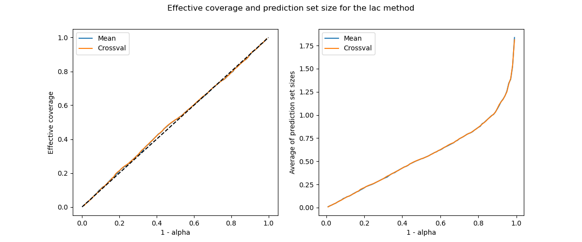
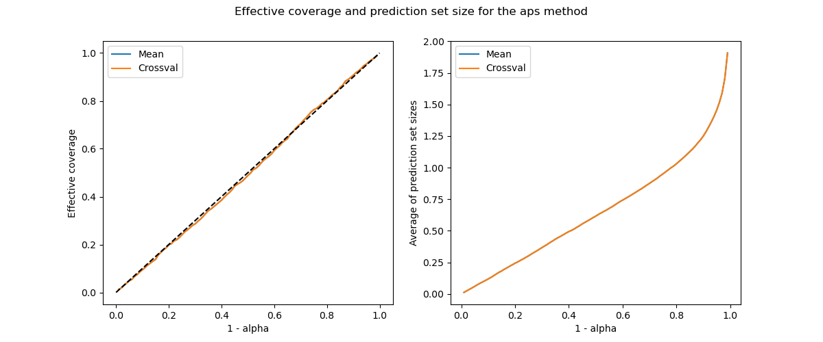
Both methods give here the same coverages and prediction set sizes for this example. In practice, we obtain very similar results for datasets containing a high number of points. This is not the case for small datasets.

The calibration plots obtained with the cross-conformal methods seem to be more robust than with the split-conformal used above. Let’s check this first impression by comparing the violation of the effective coverage from the target coverage between the cross-conformal and split-conformal methods.

violations_df = pd.DataFrame(
    index=["lac", "aps"],
    columns=["cv_mean", "cv_crossval", "splits"]
)
violations_df.loc["lac", "cv_mean"] = violations["score_cv_mean"]
violations_df.loc["lac", "cv_crossval"] = violations["score_cv_crossval"]
violations_df.loc["lac", "splits"] = np.stack(
    [
        np.abs(cov - (1 - alpha)).mean()
        for cov in split_coverages[0]
    ]
).mean()
violations_df.loc["aps", "cv_mean"] = (
    violations["cum_score_cv_mean"]
)
violations_df.loc["aps", "cv_crossval"] = (
    violations["cum_score_cv_crossval"]
)
violations_df.loc["aps", "splits"] = np.stack(
    [
        np.abs(cov - (1 - alpha)).mean()
        for cov in split_coverages[1]
    ]
).mean()

print(violations_df)

Out:

      cv_mean cv_crossval    splits
lac  0.006921     0.00748  0.014895
aps  0.007629    0.007246   0.01775