Group-conditional prediction sets¶

This example shows how to use :class:~mapie.conditional_conformal_prediction.ConditionalSplitConformalClassifier to build prediction sets with conditional guarantees on pre-defined groups.

It is inspired by the synthetic examples from Gibbs, Cherian and Candès (2023) and their conditional-conformal reference implementation. The key idea is to provide a basis function feature_map that identifies the covariate groups on which coverage should be controlled.

import matplotlib.pyplot as plt
import numpy as np
from sklearn.linear_model import LogisticRegression

from mapie.classification import SplitConformalClassifier
from mapie.conditional_conformal_prediction import ConditionalSplitConformalClassifier
from mapie.metrics.classification import (
    classification_coverage_score,
    classification_mean_width_score,
)
from mapie.utils import train_conformalize_test_split

1. Generate grouped classification data¶

The first feature is a difficulty index split into three groups. Labels are almost deterministic when this feature is small and much noisier when it is large. The second feature is the class signal. This creates groups with very different conformity-score distributions, which is exactly where marginal split conformal prediction can hide local undercoverage.

bins = np.linspace(0, 1, 4)


def generate_grouped_classification_data(n_samples=2400, random_state=10):
    rng = np.random.default_rng(random_state)
    difficulty = rng.uniform(0, 1, size=n_samples)
    signal = rng.normal(size=n_samples)

    group = np.digitize(difficulty, bins[1:-1], right=False)
    temperature = np.array([0.25, 0.70, 3.20])[group]

    logits = (
        np.column_stack([4 * signal, -4 * signal, np.zeros(n_samples)])
        / temperature[:, np.newaxis]
    )
    logits -= logits.max(axis=1, keepdims=True)
    probabilities = np.exp(logits)
    probabilities /= probabilities.sum(axis=1, keepdims=True)

    y = np.array([rng.choice(3, p=probability) for probability in probabilities])
    X = np.column_stack([difficulty, signal])
    return X, y


X, y = generate_grouped_classification_data()

(
    X_train,
    X_conformalize,
    X_test,
    y_train,
    y_conformalize,
    y_test,
) = train_conformalize_test_split(
    X,
    y,
    train_size=0.35,
    conformalize_size=0.45,
    test_size=0.20,
    random_state=10,
)

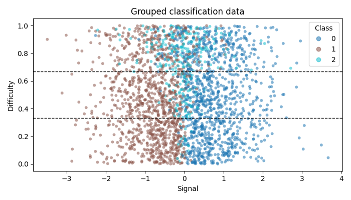
2. Plot the data¶

The plot below shows the generated samples. The horizontal dashed lines mark the three difficulty groups used by the conditional conformal procedure.

fig, ax = plt.subplots(figsize=(7, 4))
scatter = ax.scatter(
    X[:, 1],
    X[:, 0],
    c=y,
    cmap="tab10",
    s=18,
    alpha=0.55,
    edgecolor="none",
)
for threshold in bins[1:-1]:
    ax.axhline(threshold, color="black", linestyle="--", linewidth=1)
ax.set_xlabel("Signal")
ax.set_ylabel("Difficulty")
ax.set_title("Grouped classification data")
ax.legend(
    *scatter.legend_elements(),
    title="Class",
    loc="upper right",
)
plt.tight_layout()
plt.show()

Grouped classification data

3. Define the conditional groups¶

feature_map returns one indicator column per difficulty bin. The conditional classifier will use these columns to calibrate score cutoffs that are valid on each group, not only on average over the full distribution.

bin_centers = (bins[:-1] + bins[1:]) / 2
bin_labels = [f"[{left:.2f}, {right:.2f})" for left, right in zip(bins[:-1], bins[1:])]
bin_labels[-1] = "[0.67, 1.00]"


def indicator_matrix(values, bin_edges):
    values = np.asarray(values).reshape(-1)
    bin_indexes = np.digitize(values, bin_edges[1:-1], right=False)
    matrix = np.zeros((len(values), len(bin_edges) - 1))
    matrix[np.arange(len(values)), bin_indexes] = 1
    return matrix


def phi_fn(X):
    return indicator_matrix(np.asarray(X)[:, 0], bins)

4. Fit marginal and conditional conformal classifiers¶

Both methods use the same fitted logistic regression model and the same conformalization data. The only difference is that ConditionalSplitConformalClassifier receives feature_map.

confidence_level = 0.95
estimator = LogisticRegression(max_iter=1000).fit(X_train, y_train)

mapie_marginal = SplitConformalClassifier(
    estimator=estimator,
    confidence_level=confidence_level,
    conformity_score="lac",
    prefit=True,
)
mapie_marginal.conformalize(X_conformalize, y_conformalize)
_, y_pred_set_marginal = mapie_marginal.predict_set(X_test)

mapie_conditional = ConditionalSplitConformalClassifier(
    phi_fn,
    estimator=estimator,
    confidence_level=confidence_level,
    conformity_score="lac",
    prefit=True,
)
mapie_conditional.conformalize(X_conformalize, y_conformalize)
_, y_pred_set_conditional = mapie_conditional.predict_set(X_test)

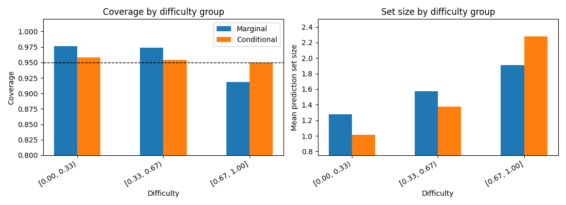
5. Evaluate and visualize the correction¶

The marginal classifier has good overall coverage, and its prediction sets already become larger as the base model gets less confident. However, the single global conformal cutoff is still not sufficient for the hardest group. The conditional classifier makes an additional group-level correction: prediction sets become smaller in easier groups and larger in the hardest group. The coverage panel below shows this correction, while the set-size panel explains where the additional uncertainty is allocated.

def group_mask(X, bin_index):
    if bin_index == len(bins) - 2:
        return (X[:, 0] >= bins[bin_index]) & (X[:, 0] <= bins[-1])
    return (X[:, 0] >= bins[bin_index]) & (X[:, 0] < bins[bin_index + 1])


def scores_by_group(y_true, y_pred_set, X):
    coverages = []
    set_sizes = []
    for bin_index in range(len(bins) - 1):
        mask = group_mask(X, bin_index)
        coverages.append(classification_coverage_score(y_true[mask], y_pred_set[mask]))
        set_sizes.append(classification_mean_width_score(y_pred_set[mask]))
    return np.asarray(coverages).ravel(), np.asarray(set_sizes).ravel()


coverage_marginal_by_group, width_marginal_by_group = scores_by_group(
    y_test, y_pred_set_marginal, X_test
)
coverage_conditional_by_group, width_conditional_by_group = scores_by_group(
    y_test, y_pred_set_conditional, X_test
)

fig, axes = plt.subplots(1, 2, figsize=(11, 4), sharex=True)
bar_width = 0.09

axes[0].bar(
    bin_centers - bar_width / 2,
    coverage_marginal_by_group,
    width=bar_width,
    label="Marginal",
)
axes[0].bar(
    bin_centers + bar_width / 2,
    coverage_conditional_by_group,
    width=bar_width,
    label="Conditional",
)
axes[0].axhline(confidence_level, color="black", linestyle="--", linewidth=1)
axes[0].set_ylim(0.80, 1.02)
axes[0].set_ylabel("Coverage")
axes[0].set_title("Coverage by difficulty group")
axes[0].legend()

axes[1].bar(
    bin_centers - bar_width / 2,
    width_marginal_by_group,
    width=bar_width,
    label="Marginal",
)
axes[1].bar(
    bin_centers + bar_width / 2,
    width_conditional_by_group,
    width=bar_width,
    label="Conditional",
)
axes[1].set_ylim(0.75, 2.50)
axes[1].set_ylabel("Mean prediction set size")
axes[1].set_title("Set size by difficulty group")

for ax in axes:
    ax.set_xlabel("Difficulty")
    ax.set_xticks(bin_centers)
    ax.set_xticklabels(bin_labels, rotation=30, ha="right")

plt.tight_layout()
plt.show()

Coverage by difficulty group, Set size by difficulty group

Total running time of the script: ( 0 minutes 0.679 seconds)

Download Python source code: plot_conditional_conformal_classification_groups.py

Download Jupyter notebook: plot_conditional_conformal_classification_groups.ipynb

Gallery generated by mkdocs-gallery