Conditional calibration with ConditionalSplitConformalRegressor¶

This example reproduces the 1D synthetic experiment of Gibbs, Cherian and Candès (2023) [1], using MAPIE's :class:~mapie.conditional_conformal_prediction.ConditionalSplitConformalRegressor.

The plot below mirrors the figure produced by the SyntheticData.ipynb notebook of the authors' reference implementation [2]: it compares a standard (marginal) split-conformal interval to the conditionally-calibrated interval on the same data and base model.

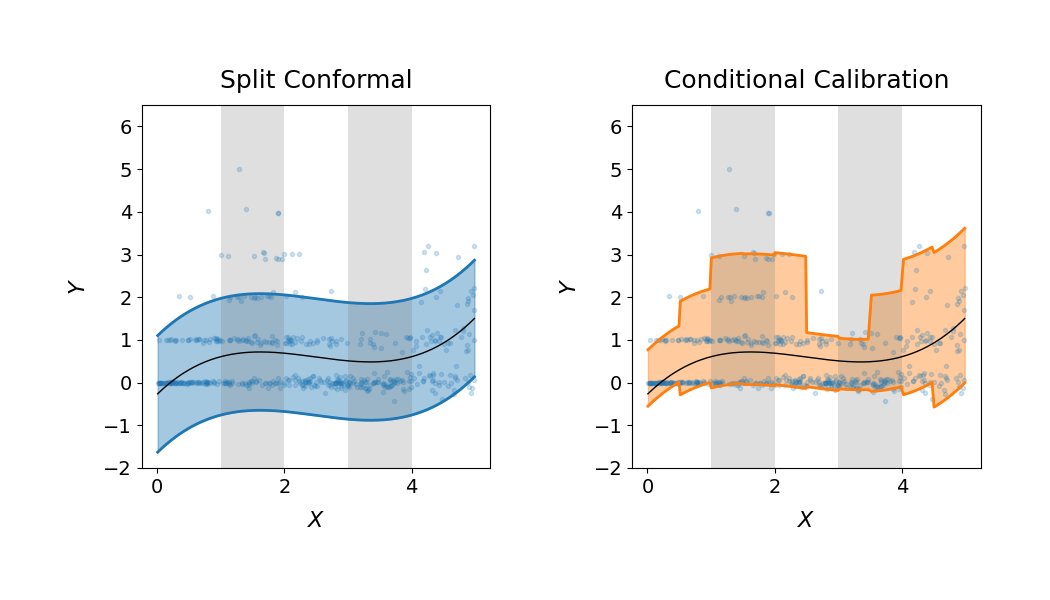
The data is heteroscedastic: the conditional spread of Y varies strongly with X. A marginal split-conformal interval uses a single score cutoff for every X, so it is too wide where the noise is small and too narrow where it is large. The conditional procedure instead guarantees coverage over a chosen finite class of covariate shifts -- here the indicators of the sub-intervals [0, 0.5), [0.5, 1), ..., [4.5, 5) -- and therefore adapts the interval width to X.

[1] Isaac Gibbs, John J. Cherian, Emmanuel J. Candès. "Conformal Prediction With Conditional Guarantees." arXiv:2305.12616, 2023.

[2] https://github.com/jjcherian/conditional-conformal

import warnings

import matplotlib.pyplot as plt
import numpy as np
import pandas as pd
import seaborn as sns
from sklearn.linear_model import LinearRegression
from sklearn.pipeline import make_pipeline
from sklearn.preprocessing import PolynomialFeatures

from mapie.conditional_conformal_prediction import ConditionalSplitConformalRegressor
from mapie.conformity_scores import AbsoluteConformityScore

warnings.filterwarnings("ignore")

Traceback (most recent call last):
  File "/home/docs/checkouts/readthedocs.org/user_builds/mapie/checkouts/latest/examples/regression/3-scientific-articles/plot_gibbs2023_conditional_conformal.py", line 35, in <module>
    import seaborn as sns
ModuleNotFoundError: No module named 'seaborn'

1. Generating the synthetic data¶

We use the exact data-generating process of the reference implementation. The mean of Y follows a smooth function of X on [0, 5], with a Poisson-like component, a small X-dependent Gaussian noise, and rare large outliers. The conditional variance is clearly heteroscedastic in X.

def generate_cqr_data(seed, n_train=2000, n_calib=1000, n_test=500):
    np.random.seed(seed)

    n_train = n_train + n_calib

    def f(x):
        """Construct data (1D example)"""
        ax = 0 * x
        for i in range(len(x)):
            ax[i] = (
                np.random.poisson(np.sin(x[i]) ** 2 + 0.1)
                + 0.03 * x[i] * np.random.randn(1)
            ).item()
            ax[i] += (
                25 * (np.random.uniform(0, 1, 1) < 0.01) * np.random.randn(1)
            ).item()
        return ax.astype(np.float32)

    x_train = np.random.uniform(0, 5.0, size=n_train).astype(np.float32)
    x_test = np.random.uniform(0, 5.0, size=n_test).astype(np.float32)

    y_train = f(x_train)
    y_test = f(x_test)

    x_train = np.reshape(x_train, (n_train, 1))
    x_test = np.reshape(x_test, (n_test, 1))

    train_set_size = len(y_train) - n_calib
    x_train_final = x_train[:train_set_size]
    x_calib = x_train[train_set_size:]
    y_train_final = y_train[:train_set_size]
    y_calib = y_train[train_set_size:]

    return x_train_final, y_train_final, x_calib, y_calib, x_test, y_test


def indicator_matrix(scalar_values, disc):
    scalar_values = np.array(scalar_values)

    # Create all possible intervals
    intervals = [(disc[i], disc[i + 1]) for i in range(len(disc) - 1)]

    # Initialize the indicator matrix
    matrix = np.zeros((len(scalar_values), len(intervals)))

    # Fill in the indicator matrix
    for i, value in enumerate(scalar_values):
        for j, (a, b) in enumerate(intervals):
            if a <= value < b:
                matrix[i, j] = 1

    return matrix


x_train_final, y_train_final, x_calib, y_calib, x_test, y_test = generate_cqr_data(
    seed=1, n_calib=2000
)

x_calib = np.asarray(x_calib, dtype=np.float64)
y_calib = np.asarray(y_calib, dtype=np.float64)

2. Fitting the base regressor¶

Following the reference experiment, the base model is a fourth-order polynomial regression. The polynomial features are wrapped in a :class:~sklearn.pipeline.Pipeline so that the estimator can be called directly on the raw covariate X: MAPIE calls predict on the raw features internally, and the conditional basis feature_map below is also defined on the raw X.

reg = make_pipeline(PolynomialFeatures(4), LinearRegression()).fit(
    x_train_final, y_train_final
)

confidence_level = 0.9
alpha = 1 - confidence_level

3. Defining the conditional guarantee¶

feature_map defines the finite-dimensional class of covariate shifts over which exact coverage is guaranteed. Here we use the indicators of the sub-intervals with endpoints in [0, 0.5, 1, ..., 5]: coverage is then valid not only marginally, but on each of these groups of X.

eps = 0.5
disc = np.arange(0, 5 + eps, eps)


def phi_fn(x):
    return indicator_matrix(x, disc)

4. Conditional calibration with MAPIE¶

We use a non-symmetric :class:~mapie.conformity_scores.AbsoluteConformityScore (the residual Y - reg.predict(X)), so that the lower and upper bounds are calibrated separately. The base model is already fitted, hence prefit=True. predict_interval solves, for each test point, a small linear program that yields the conditionally-valid score cutoff.

mapie_conditional = ConditionalSplitConformalRegressor(
    phi_fn,
    estimator=reg,
    prefit=True,
    confidence_level=confidence_level,
    conformity_score=AbsoluteConformityScore(sym=False),
)
mapie_conditional.conformalize(x_calib, y_calib)

n_test = len(x_test)
lbs = np.zeros((n_test,))
ubs = np.zeros((n_test,))
for i, x_t in enumerate(x_test):
    _, interval = mapie_conditional.predict_interval(x_t.reshape(1, -1))
    lbs[i] = interval[0, 0, 0]
    ubs[i] = interval[0, 1, 0]

5. Marginal split-conformal baseline¶

As a reference, we also compute the standard split-conformal interval, which uses a single marginal quantile of the absolute residuals on the calibration set. This interval has constant half-width q for every X.

q = np.quantile(
    np.abs(reg.predict(x_calib) - y_calib),
    np.ceil((len(x_calib) + 1) * confidence_level) / len(x_calib),
)

6. Comparing the two intervals¶

The left panel shows the marginal split-conformal interval (constant width). The right panel shows the conditional calibration: the interval narrows where the conditional noise is small and widens where it is large, while keeping the target coverage on each of the highlighted groups of X. This reproduces the figure of the original implementation [2].

sns.set(font="DejaVu Sans")
sns.set_style("whitegrid", {"axes.grid": False})
cp = sns.color_palette()
fig = plt.figure()
fig.set_size_inches(10.5, 6)

sort_order = np.argsort(x_test[0:n_test, 0])
x_test_s = x_test[sort_order]
y_test_s = y_test[sort_order]
y_test_hat = reg.predict(x_test[sort_order])
lb = lbs[sort_order]
ub = ubs[sort_order]

ax1 = fig.add_subplot(1, 2, 1)
ax1.plot(x_test_s, y_test_s, ".", alpha=0.2)
ax1.plot(x_test_s, y_test_hat, lw=1, color="k")
ax1.plot(x_test_s, y_test_hat + q, color=cp[0], lw=2)
ax1.plot(x_test_s, y_test_hat - q, color=cp[0], lw=2)
ax1.fill_between(
    x_test_s.flatten(),
    y_test_hat - q,
    y_test_hat + q,
    color=cp[0],
    alpha=0.4,
    label="split prediction interval",
)
ax1.set_ylim(-2, 6.5)
ax1.tick_params(axis="both", which="major", labelsize=14)
ax1.set_xlabel("$X$", fontsize=16, labelpad=10)
ax1.set_ylabel("$Y$", fontsize=16, labelpad=10)
ax1.set_title("Split Conformal", fontsize=18, pad=12)
ax1.axvspan(1, 2, facecolor="grey", alpha=0.25)
ax1.axvspan(3, 4, facecolor="grey", alpha=0.25)

ax2 = fig.add_subplot(1, 2, 2, sharex=ax1, sharey=ax1)
ax2.plot(x_test_s, y_test_s, ".", alpha=0.2)
ax2.plot(x_test_s, y_test_hat, color="k", lw=1)
ax2.plot(x_test_s, ub, color=cp[1], lw=2)
ax2.plot(x_test_s, lb, color=cp[1], lw=2)
ax2.fill_between(
    x_test_s.flatten(),
    lb,
    ub,
    color=cp[1],
    alpha=0.4,
    label="conditional calibration",
)
ax2.tick_params(axis="both", which="major", direction="out", labelsize=14)
ax2.set_xlabel("$X$", fontsize=16, labelpad=10)
ax2.set_ylabel("$Y$", fontsize=16, labelpad=10)
ax2.set_title("Conditional Calibration", fontsize=18, pad=12)
ax2.axvspan(1, 2, facecolor="grey", alpha=0.25)
ax2.axvspan(3, 4, facecolor="grey", alpha=0.25)

plt.tight_layout(pad=5)
plt.show()

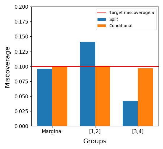
7. Group-conditional miscoverage over repeated trials¶

We now quantify the coverage difference between the two methods. Following the reference notebook [2], we repeat the experiment over independent draws of the calibration and test sets (keeping the fitted base model), and measure the miscoverage rate of both methods, marginally and on the two highlighted groups X in [1, 2] and X in [3, 4]. The conditional procedure is run with randomize=True so that its coverage is exact rather than conservative.

Both methods control the marginal miscoverage at the nominal 10% level (red line), but the split-conformal interval (blue, as in the figure above) undercovers on [1, 2] -- where the noise is large -- and overcovers on [3, 4] -- where it is small. The conditional calibration (orange) achieves the nominal miscoverage on both groups. The original experiment uses 500 trials; we use fewer here to keep the runtime of the example reasonable.

n_trials = 20
rows = []
for seed in range(n_trials):
    _, _, x_calib_t, y_calib_t, x_test_t, y_test_t = generate_cqr_data(
        seed=seed, n_calib=2000
    )
    x_calib_t = np.asarray(x_calib_t, dtype=np.float64)
    y_calib_t = np.asarray(y_calib_t, dtype=np.float64)
    x_test_t = np.asarray(x_test_t, dtype=np.float64)

    mapie_trial = ConditionalSplitConformalRegressor(
        phi_fn,
        estimator=reg,
        prefit=True,
        confidence_level=confidence_level,
        conformity_score=AbsoluteConformityScore(sym=False),
        randomize=True,
        seed=seed,
    ).conformalize(x_calib_t, y_calib_t)
    _, intervals = mapie_trial.predict_interval(x_test_t)
    miscover_conditional = (y_test_t < intervals[:, 0, 0]) | (
        y_test_t > intervals[:, 1, 0]
    )

    q_t = np.quantile(
        np.abs(reg.predict(x_calib_t) - y_calib_t),
        np.ceil((len(x_calib_t) + 1) * confidence_level) / len(x_calib_t),
    )
    miscover_split = np.abs(reg.predict(x_test_t) - y_test_t) >= q_t

    x_t = x_test_t[:, 0]
    groups = {
        "Marginal": np.ones_like(x_t, dtype=bool),
        "[1,2]": (x_t > 1) & (x_t < 2),
        "[3,4]": (x_t > 3) & (x_t < 4),
    }
    for method, miscover in [
        ("Split", miscover_split),
        ("Conditional", miscover_conditional),
    ]:
        for group_name, mask in groups.items():
            rows.append(
                {
                    "Method": method,
                    "Groups": group_name,
                    "Miscoverage": miscover[mask].mean(),
                }
            )

coverage_data = pd.DataFrame(rows)

fig, ax3 = plt.subplots(figsize=(5.5, 5))
barplot = sns.barplot(coverage_data, x="Groups", y="Miscoverage", hue="Method", ax=ax3)
barplot.axhline(alpha, color="red", label=r"Target miscoverage $\alpha$")
ax3.legend()
ax3.set_ylabel("Miscoverage", fontsize=16, labelpad=10)
ax3.set_xlabel("Groups", fontsize=16, labelpad=10)
ax3.set_ylim(0.0, 0.2)
ax3.tick_params(axis="both", which="major", labelsize=12)
plt.tight_layout()
plt.show()

Total running time of the script: ( 0 minutes 0.002 seconds)

Download Python source code: plot_gibbs2023_conditional_conformal.py

Download Jupyter notebook: plot_gibbs2023_conditional_conformal.ipynb

Gallery generated by mkdocs-gallery