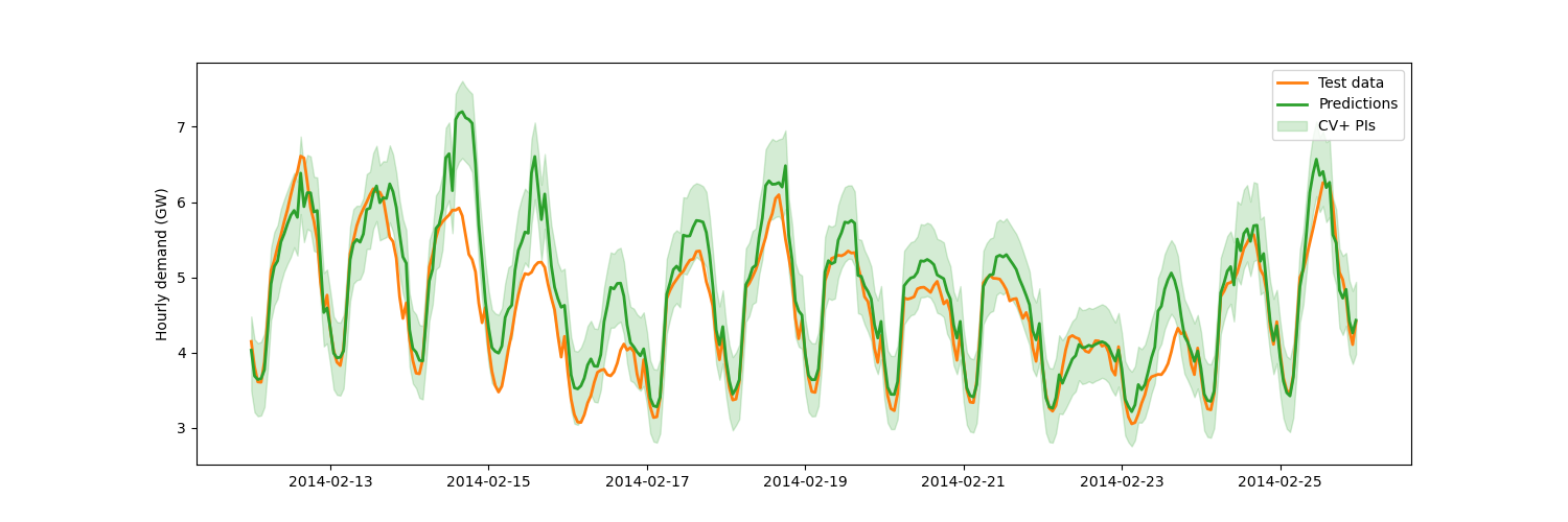
Estimating prediction intervals of time series forecast

This example uses MapieRegressor to estimate prediction intervals associated with time series forecast. We use the standard cross-validation approach to estimate conformity scores and associated prediction intervals.

We use here the Victoria electricity demand dataset used in the book “Forecasting: Principles and Practice” by R. J. Hyndman and G. Athanasopoulos. The electricity demand features daily and weekly seasonalities and is impacted by the temperature, considered here as a exogeneous variable.

The data is modelled by a Random Forest model with a RandomizedSearchCV using a sequential TimeSeriesSplit cross validation, in which the training set is prior to the validation set. The best model is then feeded into MapieRegressor to estimate the associated prediction intervals. We consider the standard CV+ resampling method.

We wish to emphasize one main limitation with this example. We use a standard cross-validation in Mapie to estimate the prediction intervals, through the sklearn.model_selection.KFold() object. Residuals are therefore estimated using models trained on data with higher indices than the validation data, which is inappropriate for time-series data. However, using a sklearn.model_selection.TimeSeriesSplit cross validation object for estimating the residuals breaks the theoretical guarantees of the Jackknife+ and CV+ methods.

Out:

/home/docs/checkouts/readthedocs.org/user_builds/mapie/conda/stable/lib/python3.10/site-packages/mapie/utils.py:598: UserWarning: WARNING: The predictions are ill-sorted.
  warnings.warn(
Coverage and prediction interval width mean for CV+: 0.815, 0.987

import pandas as pd
from matplotlib import pylab as plt
from scipy.stats import randint
from sklearn.ensemble import RandomForestRegressor
from sklearn.model_selection import RandomizedSearchCV, TimeSeriesSplit

from mapie.metrics import (regression_coverage_score,
                           regression_mean_width_score)
from mapie.regression import MapieRegressor

# Load input data and feature engineering
demand_df = pd.read_csv(
    "../../data/demand_temperature.csv", parse_dates=True, index_col=0
)
demand_df["Date"] = pd.to_datetime(demand_df.index)
demand_df["Weekofyear"] = demand_df.Date.dt.isocalendar().week.astype("int64")
demand_df["Weekday"] = demand_df.Date.dt.isocalendar().day.astype("int64")
demand_df["Hour"] = demand_df.index.hour

# Train/validation/test split
num_test_steps = 24 * 7 * 2
demand_train = demand_df.iloc[:-num_test_steps, :].copy()
demand_test = demand_df.iloc[-num_test_steps:, :].copy()
X_train = demand_train.loc[:, ["Weekofyear", "Weekday", "Hour", "Temperature"]]
y_train = demand_train["Demand"]
X_test = demand_test.loc[:, ["Weekofyear", "Weekday", "Hour", "Temperature"]]
y_test = demand_test["Demand"]

# CV parameter search
n_iter = 10
n_splits = 5
tscv = TimeSeriesSplit(n_splits=n_splits)
random_state = 59
rf_model = RandomForestRegressor(random_state=random_state)
rf_params = {"max_depth": randint(2, 30), "n_estimators": randint(10, 1e3)}
cv_obj = RandomizedSearchCV(
    rf_model,
    param_distributions=rf_params,
    n_iter=n_iter,
    cv=tscv,
    scoring="neg_root_mean_squared_error",
    random_state=random_state,
    verbose=0,
    n_jobs=-1,
)
cv_obj.fit(X_train, y_train)
best_est = cv_obj.best_estimator_

# Estimate prediction intervals on test set with best estimator
# Here, a non-nested CV approach is used for the sake of computational
# time, but a nested CV approach is preferred.
# See the dedicated example in the gallery for more information.
alpha = 0.1
mapie = MapieRegressor(
    best_est, method="plus", cv=n_splits, agg_function="median", n_jobs=-1
)
mapie.fit(X_train, y_train)
y_pred, y_pis = mapie.predict(X_test, alpha=alpha)
coverage = regression_coverage_score(y_test, y_pis[:, 0, 0], y_pis[:, 1, 0])
width = regression_mean_width_score(y_pis[:, 0, 0], y_pis[:, 1, 0])

# Print results
print(
    "Coverage and prediction interval width mean for CV+: "
    f"{coverage:.3f}, {width:.3f}"
)

# Plot estimated prediction intervals on test set
fig = plt.figure(figsize=(15, 5))
ax = fig.add_subplot(1, 1, 1)
ax.set_ylabel("Hourly demand (GW)")
ax.plot(demand_test.Demand, lw=2, label="Test data", c="C1")
ax.plot(demand_test.index, y_pred, lw=2, c="C2", label="Predictions")
ax.fill_between(
    demand_test.index,
    y_pis[:, 0, 0],
    y_pis[:, 1, 0],
    color="C2",
    alpha=0.2,
    label="CV+ PIs",
)
ax.legend()
plt.show()