Theoretical Description
There are mainly three different ways to handle uncertainty quantification in binary classification:
calibration (see Theoretical Description), confidence interval (CI) for the probability
 and prediction sets (see Theoretical Description).
These 3 notions are tightly related for score-based classifier, as it is shown in [1].
and prediction sets (see Theoretical Description).
These 3 notions are tightly related for score-based classifier, as it is shown in [1].
Prediction sets can be computed in the same way for multiclass and binary classification with
MapieClassifier, and there are the same theoretical guarantees.
Nevertheless, prediction sets are often much less informative in the binary case than in the multiclass case.
From Gupta et al [1]:
PSs and CIs are only ‘informative’ if the sets or intervals produced by them are small. To quantify this, we measure CIs using their width (denoted as
, and PSs using their diameter (defined as the width of the convex hull of the PS). For example, in the case of binary classification, the diameter of a PS is
if the prediction set is
, and
otherwise (since
always holds, the set
is more informative than a wider one such as
.
In a few words, what you need to remember about these concepts :
Calibration is useful for transforming a score (typically given by an ML model) into the probability of making a good prediction.
Set Prediction gives the set of likely predictions with a probabilistic guarantee that the true label is in this set.
Probabilistic Prediction gives a confidence interval for the predictive distribution.
1. Set Prediction
- Definition 1 (Prediction Set (PS) w.r.t
 ) [1].
 Fix a predictor
![\hat{\mu}:\mathcal{X} \to [0, 1]](_images/math/0fa4f9edb7dc59d4c5b24a297fa86b594ddf349d.png) and let
and let  .
Define the set of all subsets of
.
Define the set of all subsets of  ,
, 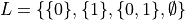 .
A function
.
A function ![S:[0,1]\to\mathcal{L}](_images/math/8c6ea09d42137d780e25085bdf5894a8509b7be9.png) is said to be
is said to be  -PS with respect to
  if:
if:

PSs are typically studied for larger output sets, such as  or
or
 .
.
See MapieClassifier to use a set predictor.
2. Probabilistic Prediction
- Definition 2 (Confidence Interval (CI) w.r.t ) [1].
Fix a predictor
and let .
Let  denote the set of all subintervals of
 ![[0,1]](_images/math/a7b17d1c3442224393b5a845ae344dbe542593d7.png) .
A function
.
A function ![C:[0,1]\to\mathcal{I}](_images/math/54e842400631e7b9072346030e37006bcc2f0bc0.png) is said to be -CI with respect to if:
is said to be -CI with respect to if:
![P(\mathbb{E}[Y|\hat{\mu}(X)]\in C(\hat{\mu}(X))) \geq 1 - \alpha](_images/math/b61a10f08075d2ccdf2781a4d3bb206f42efcb46.png)
3. Calibration
Usually, calibration is understood as perfect calibration meaning (see Theoretical Description). In practice, it is more reasonable to consider approximate calibration.
- Definition 3 (Approximate calibration) [1].
Fix a predictor
and let .
The predictor is  -calibrated
for some
-calibrated
for some ![\epsilon,\alpha\in[0, 1]](_images/math/7100248079a280c34bcd107ad30150aaf7ae764c.png) if with probability at least
if with probability at least  :
:
![|\mathbb{E}[Y|\hat{\mu}(X)] - \hat{\mu}(X)| \leq \epsilon](_images/math/8b8e295ddfe71b0e02995480d791df8ea4274f2a.png)
See CalibratedClassifierCV or MapieCalibrator
to use a calibrator.
In the CP framework, it is worth noting that Venn predictors produce probability-type predictions for the labels of test objects which are guaranteed to be well-calibrated under the standard assumption that the observations are generated independently from the same distribution [2].
4. References
[1] Gupta, Chirag, Aleksandr Podkopaev, and Aaditya Ramdas. “Distribution-free binary classification: prediction sets, confidence intervals, and calibration.” Advances in Neural Information Processing Systems 33 (2020): 3711-3723.
[2] Vovk, Vladimir, Alexander Gammerman, and Glenn Shafer. “Algorithmic Learning in a Random World.” Springer Nature, 2022.