Testing for calibration in binary classification settings

This example uses kolmogorov_smirnov_pvalue() to test for calibration of scores output by binary classifiers. Other alternatives are kuiper_pvalue() and spieglehalter_pvalue().

These statistical tests are based on the following references:

[1] Arrieta-Ibarra I, Gujral P, Tannen J, Tygert M, Xu C. Metrics of calibration for probabilistic predictions. The Journal of Machine Learning Research. 2022 Jan 1;23(1):15886-940.

[2] Tygert M. Calibration of P-values for calibration and for deviation of a subpopulation from the full population. arXiv preprint arXiv:2202.00100. 2022 Jan 31.

[3] D. A. Darling. A. J. F. Siegert. The First Passage Problem for a Continuous Markov Process. Ann. Math. Statist. 24 (4) 624 - 639, December, 1953.

import numpy as np
from matplotlib import pyplot as plt
from sklearn.utils import check_random_state

from mapie._typing import NDArray
from mapie.metrics import (cumulative_differences, kolmogorov_smirnov_p_value,
                           length_scale)

1. Create 1-dimensional dataset and scores to test for calibration

We start by simulating a 1-dimensional binary classification problem. We assume that the ground truth probability is driven by a sigmoid function, and we generate label according to this probability distribution.

def sigmoid(x: NDArray):
    y = 1 / (1 + np.exp(-x))
    return y


def generate_y_true_calibrated(
    y_prob: NDArray,
    random_state: int = 1
) -> NDArray:
    generator = check_random_state(random_state)
    uniform = generator.uniform(size=len(y_prob))
    y_true = (uniform <= y_prob).astype(float)
    return y_true


X = np.linspace(-5, 5, 2000)
y_prob = sigmoid(X)
y_true = generate_y_true_calibrated(y_prob)

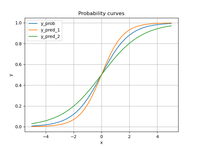
Next we provide two additional miscalibrated scores (on purpose).

y = {
    "y_prob": y_prob,
    "y_pred_1": sigmoid(1.3*X),
    "y_pred_2": sigmoid(0.7*X)
}

This is how the two miscalibration curves stands next to the ground truth.

for name, y_score in y.items():
    plt.plot(X, y_score, label=name)
plt.title("Probability curves")
plt.xlabel("x")
plt.ylabel("y")
plt.grid()
plt.legend()
plt.show()

Alternatively, you can readily see how much there is miscalibration in this view where we plot scores against the ground truth probability.

for name, y_score in y.items():
    plt.plot(y_prob, y_score, label=name)
plt.title("Probability curves")
plt.xlabel("True probability")
plt.ylabel("Estimated probability")
plt.grid()
plt.legend()
plt.show()

2. Visualizing and testing for miscalibration

We leverage the Kolomogorov-Smirnov statistical test kolmogorov_smirnov_pvalue(). It is based on the cumulative difference between sorted scores and labels. If the null hypothesis holds (i.e., the scores are well calibrated), the curve of the cumulative differences share some nice properties with the standard Brownian motion, in particular its range and maximum absolute value [1, 2].

Let’s have a look.

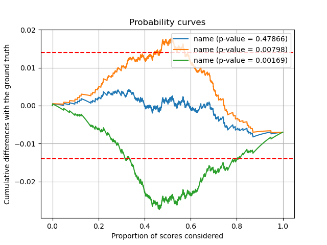
First we compute the cumulative differences.

cum_diffs = {
    name: cumulative_differences(y_true, y_score)
    for name, y_score in y.items()
}

We want to plot is along the proportion of scores taken into account.

k = np.arange(len(y_true))/len(y_true)

We also want to compare the extension of the curve to that of a typical Brownian motion.

sigma = length_scale(y_prob)

Finally, we compute the p-value according to Kolmogorov-Smirnov test [2, 3].

p_values = {
    name: kolmogorov_smirnov_p_value(y_true, y_score)
    for name, y_score in y.items()
}

The graph hereafter shows cumulative differences of each series of scores. The horizontal bars are typical length scales expected if the null hypothesis holds (standard Brownian motion). You can see that our two miscalibrated scores overshoot these limits, and that their p-values are accordingly very small. On the contrary, you can see that the well calibrated ground truth perfectly lies within the expected bounds with a p-value close to 1.

So we conclude by both visual and statistical arguments that we reject the null hypothesis for the two miscalibrated scores !

for name, cum_diff in cum_diffs.items():
    plt.plot(k, cum_diff, label=f"name (p-value = {p_values[name]:.5f})")
plt.axhline(y=2*sigma, color="r", linestyle="--")
plt.axhline(y=-2*sigma, color="r", linestyle="--")
plt.title("Probability curves")
plt.xlabel("Proportion of scores considered")
plt.ylabel("Cumulative differences with the ground truth")
plt.grid()
plt.legend()
plt.show()