Evaluating the asymptotic convergence of p-values

This example uses kolmogorov_smirnov_pvalue(), kuiper_pvalue() and spieglehalter_pvalue(). We investigate the asymptotic convergence of these functions toward real p-values. Indeed, these quantities are only asymptotic p-values, i.e. when the number of observations is infinite. However, they can be safely used as real p-values even with moderate dataset sizes. This is what we are going to illustrate in this exampple.

To this end, we generate many datasets that are calibrated by nature, and plot the distribution of the p-values. A p-value must follow a uniform distribution when computed on statistical samples following the null hypothesis.

The argument can be retrieved from the following references:

[1] Arrieta-Ibarra I, Gujral P, Tannen J, Tygert M, Xu C. Metrics of calibration for probabilistic predictions. The Journal of Machine Learning Research. 2022 Jan 1;23(1):15886-940.

[2] Tygert M. Calibration of P-values for calibration and for deviation of a subpopulation from the full population. arXiv preprint arXiv:2202.00100. 2022 Jan 31.

[3] D. A. Darling. A. J. F. Siegert. The First Passage Problem for a Continuous Markov Process. Ann. Math. Statist. 24 (4) 624 - 639, December, 1953.

import numpy as np
from matplotlib import pyplot as plt
from sklearn.utils import check_random_state

from mapie._typing import NDArray
from mapie.metrics import (kolmogorov_smirnov_p_value, kuiper_p_value,
                           spiegelhalter_p_value)

First we need to generate scores that are perfecty calibrated. To do so, we simply start from a given array of probabilities between 0 and 1, and draw random labels 0 or 1 according to these probabilities.

def generate_y_true_calibrated(
    y_prob: NDArray,
    random_state: int = 1
) -> NDArray:
    generator = check_random_state(random_state)
    uniform = generator.uniform(size=len(y_prob))
    y_true = (uniform <= y_prob).astype(float)
    return y_true

Then, we draw many different calibrated datasets, each with a fixed dataset size. For each of these datasets, we compute the available p-values implemented in MAPIE.

n_sets = 10000
n_points = 500
ks_p_values = []
ku_p_values = []
sp_p_values = []
for i in range(n_sets):
    y_score = np.linspace(0, 1, n_points)
    y_true = generate_y_true_calibrated(y_score, random_state=i)
    ks_p_value = kolmogorov_smirnov_p_value(y_true, y_score)
    ku_p_value = kuiper_p_value(y_true, y_score)
    sp_p_value = spiegelhalter_p_value(y_true, y_score)
    ks_p_values.append(ks_p_value)
    ku_p_values.append(ku_p_value)
    sp_p_values.append(sp_p_value)
ks_p_values = np.sort(ks_p_values)
ku_p_values = np.sort(ku_p_values)
sp_p_values = np.sort(sp_p_values)

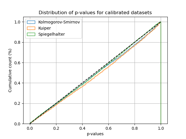
Finally, we plot the empirical cumulative distribution function of the p-values computed on these many datasets. We see that even for moderately sized datasets, the p-values computed closely follow the expected uniform distribution under the null hypothesis. It appears that Kuiper p-value is the slowest to converge compared to Spiegelhalter and Kolmogorov-Smirnov.

plt.hist(
    ks_p_values, 100,
    cumulative=True, density=True, histtype="step", label="Kolmogorov-Smirnov"
)
plt.hist(
    ku_p_values, 100,
    cumulative=True, density=True, histtype="step", label="Kuiper"
)
plt.hist(
    sp_p_values, 100,
    cumulative=True, density=True, histtype="step", label="Spiegelhalter"
)
plt.plot([0, 1], [0, 1], "--", color="black")
plt.title("Distribution of p-values for calibrated datasets")
plt.xlabel("p-values")
plt.ylabel("Cumulative count (%)")
plt.grid()
plt.legend()
plt.show()