Tutorial for residual normalised score

We will use the sklearn california housing dataset to understand how the residual normalised score works and show the multiple ways of using it.

We will explicit the experimental setup below.

import warnings

import matplotlib.pyplot as plt
import numpy as np
from matplotlib.ticker import FormatStrFormatter
from numpy.typing import ArrayLike
from sklearn.datasets import fetch_california_housing
from sklearn.ensemble import RandomForestRegressor
from sklearn.linear_model import LinearRegression
from sklearn.model_selection import train_test_split

from mapie.conformity_scores import ResidualNormalisedScore
from mapie.metrics import regression_coverage_score_v2, regression_ssc_score
from mapie.regression import MapieRegressor

warnings.filterwarnings("ignore")

random_state = 23
rng = np.random.default_rng(random_state)
round_to = 3

1. Data

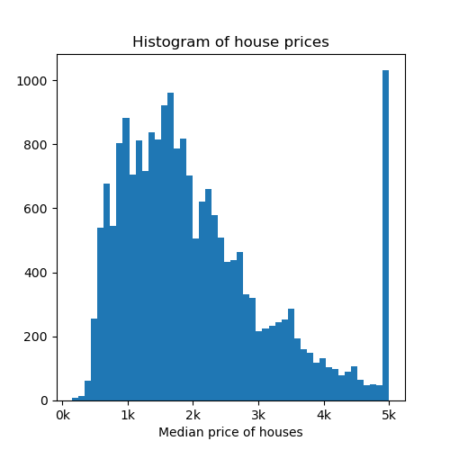
The target variable of this dataset is the median house value for the California districts. This dataset is composed of 8 features, including variables such as the age of the house, the median income of the neighborhood, the average number of rooms or bedrooms or even the location in latitude and longitude. In total there are around 20k observations.

data = fetch_california_housing()
X = data.data
y = data.target

Now let’s visualize a histogram of the price of the houses.

fig, axs = plt.subplots(1, 1, figsize=(5, 5))
axs.hist(y, bins=50)
axs.set_xlabel("Median price of houses")
axs.set_title("Histogram of house prices")
axs.xaxis.set_major_formatter(FormatStrFormatter('%.0f' + "k"))
plt.show()

Let’s now create the different splits for the dataset, with a training, calibration, residual and test set. Recall that the calibration set is used for calibrating the prediction intervals and the residual set is used to fit the residual estimator used by the ResidualNormalisedScore.

np.array(X)
np.array(y)
X_train, X_test, y_train, y_test = train_test_split(
    X,
    y,
    random_state=random_state,
    test_size=0.02
)
X_train, X_calib, y_train, y_calib = train_test_split(
    X_train,
    y_train,
    random_state=random_state
)
X_calib_prefit, X_res, y_calib_prefit, y_res = train_test_split(
    X_calib,
    y_calib,
    random_state=random_state,
    test_size=0.5
)

2. Models

We will now define 4 different ways of using the residual normalised score. Remember that this score is only available in the split setup. First, the simplest one with all the default parameters : a LinearRegression is used for the residual estimator. (Note that to avoid negative values it is trained with the log of the features and the exponential of the predictions are used). It is also possible to use it with cv="prefit" i.e. with the base model trained beforehand. The third setup that we illustrate here is with the residual model prefitted : we can set the estimator in parameters of the class, not forgetting to specify prefit="True". Finally, as an example of the exotic parameterisation we can do : we use as a residual estimator a LinearRegression wrapped to avoid negative values like it is done by default in the class.

class PosEstim(LinearRegression):
    def __init__(self):
        super().__init__()

    def fit(self, X, y):
        super().fit(
            X, np.log(np.maximum(y, np.full(y.shape, np.float64(1e-8))))
        )
        return self

    def predict(self, X):
        y_pred = super().predict(X)
        return np.exp(y_pred)


base_model = RandomForestRegressor(n_estimators=10, random_state=random_state)
base_model = base_model.fit(X_train, y_train)

residual_estimator = RandomForestRegressor(
    n_estimators=20,
    max_leaf_nodes=70,
    min_samples_leaf=7,
    random_state=random_state
)
residual_estimator = residual_estimator.fit(
    X_res, np.abs(np.subtract(y_res, base_model.predict(X_res)))
)
wrapped_residual_estimator = PosEstim().fit(
    X_res, np.abs(np.subtract(y_res, base_model.predict(X_res)))
)
# Estimating prediction intervals
STRATEGIES = {
    "Default": {
        "cv": "split",
        "conformity_score": ResidualNormalisedScore()
    },
    "Base model prefit": {
        "cv": "prefit",
        "estimator": base_model,
        "conformity_score": ResidualNormalisedScore(
            split_size=0.5, random_state=random_state
        )
    },
    "Base and residual model prefit": {
        "cv": "prefit",
        "estimator": base_model,
        "conformity_score": ResidualNormalisedScore(
            residual_estimator=residual_estimator,
            random_state=random_state,
            prefit=True
        )
    },
    "Wrapped residual model": {
        "cv": "prefit",
        "estimator": base_model,
        "conformity_score": ResidualNormalisedScore(
            residual_estimator=wrapped_residual_estimator,
            random_state=random_state,
            prefit=True
        )
    },
}

y_pred, intervals, coverage, cond_coverage = {}, {}, {}, {}
num_bins = 10
alpha = 0.1
for strategy, params in STRATEGIES.items():
    mapie = MapieRegressor(**params, random_state=random_state)
    if mapie.conformity_score.prefit:
        mapie.fit(X_calib_prefit, y_calib_prefit)
    else:
        mapie.fit(X_calib, y_calib)
    y_pred[strategy], intervals[strategy] = mapie.predict(X_test, alpha=alpha)

    coverage[strategy] = regression_coverage_score_v2(
        y_test, intervals[strategy]
    )
    cond_coverage[strategy] = regression_ssc_score(
        y_test, intervals[strategy], num_bins=num_bins
    )


def yerr(y_pred, intervals) -> ArrayLike:
    """
    Returns the error bars with the point prediction and its interval

    Parameters
    ----------
    y_pred: ArrayLike
        Point predictions.
    intervals: ArrayLike
        Predictions intervals.

    Returns
    -------
    ArrayLike
        Error bars.
    """
    return np.abs(np.concatenate(
        [
            np.expand_dims(y_pred, 0) - intervals[:, 0, 0].T,
            intervals[:, 1, 0].T - np.expand_dims(y_pred, 0),
        ],
        axis=0,
    ))


def plot_predictions(y, y_pred, intervals, coverage, cond_coverage, ax=None):
    """
    Plots y_true against y_pred with the associated interval.

    Parameters
    ----------
    y: ArrayLike
       Observed targets
    y_pred: ArrayLike
       Predictions
    intervals: ArrayLike
       Prediction intervals
    coverage: float
       Global coverage
    cond_coverage: float
        Maximum violation coverage
    ax: matplotlib axes
       An ax can be provided to include this plot in a subplot
    """
    if ax is None:
        fig, ax = plt.subplots(figsize=(6, 5))

    ax.set_xlim([-0.5, 5.5])
    ax.set_ylim([-0.5, 5.5])

    error = y_pred - intervals[:, 0, 0]
    warning1 = y_test > y_pred + error
    warning2 = y_test < y_pred - error
    warnings = warning1 + warning2
    ax.errorbar(
        y[~warnings],
        y_pred[~warnings],
        yerr=np.abs(error[~warnings]),
        color="g",
        alpha=0.2,
        linestyle="None",
        label="Inside prediction interval"
    )
    ax.errorbar(
        y[warnings],
        y_pred[warnings],
        yerr=np.abs(error[warnings]),
        color="r",
        alpha=0.3,
        linestyle="None",
        label="Outside prediction interval"
    )

    ax.scatter(y, y_pred, s=3, color="black")
    ax.plot([0, max(max(y), max(y_pred))], [0, max(max(y), max(y_pred))], "-r")
    ax.set_title(
        f"{strategy} - coverage={coverage:.0%} " +
        f"- max violation={cond_coverage:.0%}"
    )
    ax.set_xlabel("y true")
    ax.set_ylabel("y pred")
    ax.legend()
    ax.grid()


fig, axs = plt.subplots(nrows=2, ncols=2, figsize=(12, 10))
for ax, strategy in zip(axs.flat, STRATEGIES.keys()):
    plot_predictions(
        y_test,
        y_pred[strategy],
        intervals[strategy],
        coverage[strategy][0],
        cond_coverage[strategy][0],
        ax=ax
    )

fig.suptitle(f"Predicted values and intervals of level {alpha}")
plt.tight_layout()
plt.show()

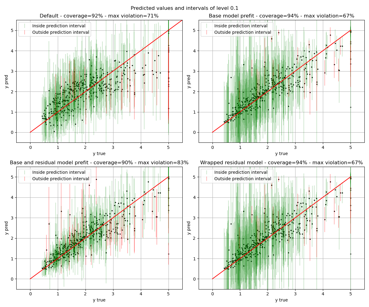
The results show that all the setups reach the global coverage guaranteed of 1-alpha. It is interesting to note that the “base model prefit” and the “wrapped residual model” give exactly the same results. And this is because they are the same models : one prefitted and one fitted directly in the class.