Note
Go to the end to download the full example code.
Defining a custom risk for binary classification
MAPIE ships with several predefined risks and performance metrics for binary classification (precision, recall, accuracy, false positive rate…). When the metric you care about is not one of them, you can define your own with BinaryRisk and control it exactly like a predefined one.
In this example, we show how to define specificity (the true negative rate) as a custom risk and use it with the BinaryClassificationController.
Specificity is the proportion of actual negatives that are correctly predicted as negative. It is a natural target in screening problems where we want to avoid raising too many alarms on healthy/benign cases, while keeping recall (the ability to catch the positive cases) as high as possible.
import matplotlib.pyplot as plt
import numpy as np
from sklearn.datasets import make_circles
from sklearn.metrics import recall_score
from sklearn.neural_network import MLPClassifier

from mapie.risk_control import BinaryClassificationController, BinaryRisk
from mapie.utils import train_conformalize_test_split

RANDOM_STATE = 42
First, load the dataset and split it into training, calibration (for conformalization), and test sets, then fit a classifier on the training data.
X, y = make_circles(n_samples=5000, noise=0.3, factor=0.3, random_state=RANDOM_STATE)
(X_train, X_calib, X_test, y_train, y_calib, y_test) = train_conformalize_test_split(
    X,
    y,
    train_size=0.7,
    conformalize_size=0.1,
    test_size=0.2,
    random_state=RANDOM_STATE,
)

clf = MLPClassifier(max_iter=150, random_state=RANDOM_STATE)
clf.fit(X_train, y_train)
Defining the custom risk
Any metric that can be written as
sum(occurrence if condition) / sum(condition) can be controlled by the
BinaryClassificationController, thanks to the Learn Then Test framework
implemented in MAPIE.
A BinaryRisk is therefore defined by two per-sample functions, both taking
the ground-truth labels y_true and the predictions y_pred and
returning boolean arrays:
risk_condition: which samples count towards the metric (the denominator),risk_occurrence: among those, which ones are a “success” (the numerator).
For specificity (true negative rate), we look at the actual negatives
(y_true == 0, the condition) and count those that are correctly predicted
as negative (y_pred == 0, the occurrence). In other words,
specificity = count(y_pred == 0 and y_true == 0) / count(y_true == 0).
Because a higher specificity is better, we set higher_is_better=True so
that MAPIE treats it as a performance metric rather than a risk.
specificity = BinaryRisk(
    risk_occurrence=lambda y_true, y_pred: y_pred == 0,
    risk_condition=lambda y_true, y_pred: y_true == 0,
    higher_is_better=True,
)
Controlling the custom risk
We now initialize a BinaryClassificationController using the probability
estimation function of the fitted estimator (clf.predict_proba), our
custom specificity risk, a target level, and a confidence level. The
controller thresholds the predicted probability of the positive class: a
higher threshold predicts fewer positives, which mechanically increases
specificity but lowers recall.
When a custom risk is used, best_predict_param_choice="auto" cannot guess
a sensible secondary objective, so we specify one explicitly. Here we maximize
recall: among all thresholds that guarantee the target specificity, the
controller selects the one that catches the most positive cases.
target_specificity = 0.8
confidence_level = 0.9
bcc = BinaryClassificationController(
    clf.predict_proba,
    specificity,
    target_level=target_specificity,
    confidence_level=confidence_level,
    best_predict_param_choice="recall",
)
bcc.calibrate(X_calib, y_calib)

print(
    f"{len(bcc.valid_predict_params)} thresholds found that guarantee a specificity "
    f"of at least {target_specificity} with a confidence of {confidence_level}.\n"
    "Among those, the one that maximizes the secondary objective (recall here) is: "
    f"{bcc.best_predict_param:.2f}."
)
60 thresholds found that guarantee a specificity of at least 0.8 with a confidence of 0.9.
Among those, the one that maximizes the secondary objective (recall here) is: 0.40.
Just like with a predefined risk, we can visualize how the threshold values impact specificity and which thresholds are statistically guaranteed.
proba_positive_class = clf.predict_proba(X_calib)[:, 1]

tested_thresholds = bcc._predict_params
specificities = np.full(len(tested_thresholds), np.inf)
for i, threshold in enumerate(tested_thresholds):
    y_pred = (proba_positive_class >= threshold).astype(int)
    # specificity is the recall of the negative class
    specificities[i] = recall_score(y_calib, y_pred, pos_label=0)

valid_thresholds_indices = np.array(
    [t in bcc.valid_predict_params for t in tested_thresholds]
)
best_threshold_index = np.where(tested_thresholds == bcc.best_predict_param)[0][0]

plt.figure()
plt.scatter(
    tested_thresholds[valid_thresholds_indices],
    specificities[valid_thresholds_indices],
    c="tab:green",
    label="Valid thresholds",
)
plt.scatter(
    tested_thresholds[~valid_thresholds_indices],
    specificities[~valid_thresholds_indices],
    c="tab:red",
    label="Invalid thresholds",
)
plt.scatter(
    tested_thresholds[best_threshold_index],
    specificities[best_threshold_index],
    c="tab:green",
    label="Best threshold",
    marker="*",
    edgecolors="k",
    s=300,
)
plt.axhline(target_specificity, color="tab:gray", linestyle="--")
plt.text(
    0.05,
    target_specificity + 0.02,
    "Target specificity",
    color="tab:gray",
    fontstyle="italic",
)
plt.xlabel("Threshold")
plt.ylabel("Specificity")
plt.legend()
plt.show()
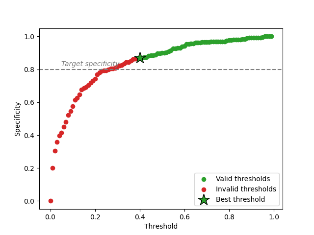
Like in the quickstart, low thresholds correspond to specificity values below the target and are therefore invalid. Some thresholds whose empirical specificity is above the target are also rejected: risk control takes a margin to account for the uncertainty due to the finite size of the calibration set, so that the guarantee holds on unseen data with high probability.
We can confirm this on the test set by using the predict method of the
controller, which applies the best threshold.
y_pred_test = bcc.predict(X_test)
test_specificity = recall_score(y_test, y_pred_test, pos_label=0)
test_recall = recall_score(y_test, y_pred_test, pos_label=1)

print(
    "With the best threshold, on the test set:\n"
    f"- specificity is {test_specificity:.3f} (target was {target_specificity}),\n"
    f"- recall is {test_recall:.3f}."
)
With the best threshold, on the test set:
- specificity is 0.809 (target was 0.8),
- recall is 0.881.
The specificity measured on the test set is close to (and above) the target,
illustrating that the guarantee obtained on the calibration set transfers to
unseen data. The same recipe applies to any binary metric that can be written
as sum(occurrence if condition) / sum(condition): define it once with
BinaryRisk, then control it with the BinaryClassificationController.
Total running time of the script: (0 minutes 4.426 seconds)