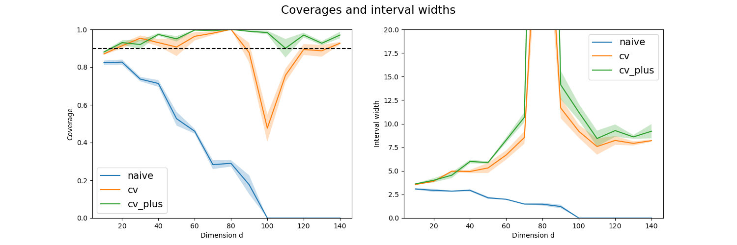
Reproducing the simulations from Foygel-Barber et al. (2020)

MapieRegressor is used to investigate the coverage level and the prediction interval width as a function of the dimension using simulated data points as introduced in Foygel-Barber et al. (2021) [1].

This simulation generates several times linear data with random noise whose signal-to-noise is equal to 10 and for several given dimensions.

Here we use MAPIE, with a LinearRegression base model, to estimate the width means and the coverage levels of the prediction intervals estimated by all the available strategies as function of the dataset dimension.

We then show the prediction interval coverages and widths as a function of the dimension values for selected strategies with standard error given by the different trials.

This simulation is carried out to emphasize the instability of the prediction intervals estimated by the jackknife strategy when the dataset dimension is equal to the number of training samples (here 100).

[1] Rina Foygel Barber, Emmanuel J. Candès, Aaditya Ramdas, and Ryan J. Tibshirani. “Predictive inference with the jackknife+.” Ann. Statist., 49(1):486–507, February 2021.

from typing import Any, Dict

import numpy as np
from matplotlib import pyplot as plt
from sklearn.linear_model import LinearRegression

from mapie._typing import NDArray
from mapie.metrics import (regression_coverage_score,
                           regression_mean_width_score)
from mapie.regression import MapieRegressor


def PIs_vs_dimensions(
    strategies: Dict[str, Any],
    alpha: float,
    n_trial: int,
    dimensions: NDArray,
) -> Dict[str, Dict[int, Dict[str, NDArray]]]:
    """
    Compute the prediction intervals for a linear regression problem.
    Function adapted from Foygel-Barber et al. (2020).

    It generates several times linear data with random noise whose
    signal-to-noise     is equal to 10 and for several given dimensions,
    given by the dimensions list.

    Here we use MAPIE, with a LinearRegression base model, to estimate
    the width means and the coverage levels of the prediction intervals
    estimated by all the available strategies as a function of
    the dataset dimension.

    This simulation is carried out to emphasize the instability
    of the prediction intervals estimated by the Jackknife strategy
    when the dataset dimension is equal to the number
    of training samples (here 100).

    Parameters
    ----------
    strategies : Dict[str, Dict[str, Any]]
        List of strategies for estimating prediction intervals,
        with corresponding parameters.
    alpha : float
        1 - (target coverage level).
    n_trial : int
        Number of trials for each dimension for estimating
        prediction intervals.
        For each trial, a new random noise is generated.
    dimensions : List[int]
        List of dimension values of input data.

    Returns
    -------
    Dict[str, Dict[int, Dict[str, NDArray]]]
        Prediction interval widths and coverages for each strategy, trial,
        and dimension value.
    """
    n_train = 100
    n_test = 100
    SNR = 10
    results: Dict[str, Dict[int, Dict[str, NDArray]]] = {
        strategy: {
            dimension: {
                "coverage": np.empty(n_trial),
                "width_mean": np.empty(n_trial),
            }
            for dimension in dimensions
        }
        for strategy in strategies
    }
    for dimension in dimensions:
        for trial in range(n_trial):
            beta = np.random.normal(size=dimension)
            beta_norm = np.sqrt(np.square(beta).sum())
            beta = beta / beta_norm * np.sqrt(SNR)
            X_train = np.random.normal(size=(n_train, dimension))
            noise_train = np.random.normal(size=n_train)
            noise_test = np.random.normal(size=n_test)
            y_train = X_train.dot(beta) + noise_train
            X_test = np.random.normal(size=(n_test, dimension))
            y_test = X_test.dot(beta) + noise_test

            for strategy, params in strategies.items():
                mapie = MapieRegressor(
                    LinearRegression(),
                    agg_function="median",
                    n_jobs=-1,
                    **params
                )
                mapie.fit(X_train, y_train)
                _, y_pis = mapie.predict(X_test, alpha=alpha)
                coverage = regression_coverage_score(
                    y_test, y_pis[:, 0, 0], y_pis[:, 1, 0]
                )
                results[strategy][dimension]["coverage"][trial] = coverage
                width_mean = regression_mean_width_score(
                    y_pis[:, 0, 0], y_pis[:, 1, 0]
                )
                results[strategy][dimension]["width_mean"][trial] = width_mean
    return results


def plot_simulation_results(
    results: Dict[str, Dict[int, Dict[str, NDArray]]], title: str
) -> None:
    """
    Show the prediction interval coverages and widths as a function
    of dimension values for selected strategies with standard error
    given by different trials.

    Parameters
    ----------
    results : Dict[str, Dict[int, Dict[str, NDArray]]]
        Prediction interval widths and coverages for each strategy, trial,
        and dimension value.
    title : str
        Title of the plot.
    """
    fig, (ax1, ax2) = plt.subplots(1, 2, figsize=(15, 5))
    plt.rcParams.update({"font.size": 14})
    plt.suptitle(title)
    for strategy in results:
        dimensions = list(results[strategy].keys())
        n_dim = len(dimensions)
        coverage_mean = np.zeros(n_dim)
        coverage_SE = np.zeros(n_dim)
        width_mean = np.zeros(n_dim)
        width_SE = np.zeros(n_dim)

        for idim, dim in enumerate(dimensions):
            coverage = results[strategy][dim]["coverage"]
            coverage_mean[idim] = coverage.mean()
            coverage_SE[idim] = coverage.std() / np.sqrt(ntrial)
            width = results[strategy][dim]["width_mean"]
            width_mean[idim] = width.mean()
            width_SE[idim] = width.std() / np.sqrt(ntrial)
        ax1.plot(dimensions, coverage_mean, label=strategy)
        ax1.fill_between(
            dimensions,
            coverage_mean - coverage_SE,
            coverage_mean + coverage_SE,
            alpha=0.25,
        )
        ax2.plot(dimensions, width_mean, label=strategy)
        ax2.fill_between(
            dimensions,
            width_mean - width_SE,
            width_mean + width_SE,
            alpha=0.25,
        )
    ax1.axhline(1 - alpha, linestyle="dashed", c="k")
    ax1.set_ylim(0.0, 1.0)
    ax1.set_xlabel("Dimension d")
    ax1.set_ylabel("Coverage")
    ax1.legend()
    ax2.set_ylim(0, 20)
    ax2.set_xlabel("Dimension d")
    ax2.set_ylabel("Interval width")
    ax2.legend()


STRATEGIES = {
    "naive": dict(method="naive"),
    "cv": dict(method="base", cv=5),
    "cv_plus": dict(method="plus", cv=5),
}
alpha = 0.1
ntrial = 3
dimensions = np.arange(10, 150, 10)
results = PIs_vs_dimensions(STRATEGIES, alpha, ntrial, dimensions)
plot_simulation_results(results, title="Coverages and interval widths")
plt.show()