Estimating conditional coverage

This example uses MapieRegressor() with conformal scores that returns adaptive intervals i.e. (GammaConformityScore and ResidualNormalisedScore) as well as MapieQuantileRegressor(). The conditional coverage is computed with the three functions that allows to estimate the conditional coverage in regression regression_ssc(), regression_ssc_score() and hsic().

import warnings
from typing import Tuple, Union

import matplotlib.pyplot as plt
import numpy as np
import pandas as pd
from lightgbm import LGBMRegressor

from mapie._typing import NDArray
from mapie.conformity_scores import (GammaConformityScore,
                                     ResidualNormalisedScore)
from mapie.metrics import (hsic, regression_coverage_score_v2, regression_ssc,
                           regression_ssc_score)
from mapie.regression import MapieQuantileRegressor, MapieRegressor
from mapie.subsample import Subsample

warnings.filterwarnings("ignore")

random_state = 42
split_size = 0.20
alpha = 0.05
rng = np.random.default_rng(random_state)


# Functions for generating our dataset
def sin_with_controlled_noise(
    min_x: Union[int, float],
    max_x: Union[int, float],
    n_samples: int,
) -> Tuple[NDArray, NDArray]:
    """
    Generate a dataset following sinx except that one interval over two 1 or -1
    (0.5 probability) is added to X

    Parameters
    ----------
    min_x: Union[int, float]
        The minimum value for X.

    max_x: Union[int, float]
        The maximum value for X.

    n_samples: int
        The number of samples wanted in the dataset.

    Returns
    -------
    Tuple[NDArray, NDArray]
        - X: feature data.
        - y: target data
    """
    X = rng.uniform(min_x, max_x, size=(n_samples, 1)).astype(np.float32)
    y = np.zeros(shape=(n_samples,))

    for i in range(int(max_x) + 1):
        indexes = np.argwhere(np.greater_equal(i, X) * np.greater(X, i - 1))
        if i % 2 == 0:
            for index in indexes:
                noise = rng.choice([-1, 1])
                y[index] = np.sin(X[index][0]) + noise * rng.random() + 2
        else:
            for index in indexes:
                y[index] = np.sin(X[index][0]) + rng.random() / 5 + 2

    return X, y


# Data generation
min_x, max_x, n_samples = 0, 10, 3000
X_train, y_train = sin_with_controlled_noise(min_x, max_x, n_samples)
X_test, y_test = sin_with_controlled_noise(min_x, max_x,
                                           int(n_samples * split_size))

# Definition of our base models
model = LGBMRegressor(random_state=random_state, alpha=0.5)
model_quant = LGBMRegressor(
            objective="quantile",
            alpha=0.5,
            random_state=random_state
)


# Definition of the experimental set up
STRATEGIES = {
    "CV+": {
        "method": "plus",
        "cv": 10,
    },
    "JK+ab_Gamma": {
        "method": "plus",
        "cv": Subsample(n_resamplings=100),
        "conformity_score": GammaConformityScore()
    },
    "ResidualNormalised": {
        "cv": "split",
        "conformity_score": ResidualNormalisedScore(
            residual_estimator=LGBMRegressor(
                alpha=0.5,
                random_state=random_state),
            split_size=0.7,
            random_state=random_state
        )
    },
    "CQR": {
        "method": "quantile", "cv": "split", "alpha": alpha
    },
}

y_pred, intervals, coverage, cond_coverage, coef_corr = {}, {}, {}, {}, {}
num_bins = 10
for strategy, params in STRATEGIES.items():
    # computing predictions
    if strategy == "CQR":
        mapie = MapieQuantileRegressor(
            model_quant,
            **params
        )
        mapie.fit(X_train, y_train, random_state=random_state)
        y_pred[strategy], intervals[strategy] = mapie.predict(X_test)
    else:
        mapie = MapieRegressor(model, **params, random_state=random_state)
        mapie.fit(X_train, y_train)
        y_pred[strategy], intervals[strategy] = mapie.predict(
            X_test, alpha=alpha
        )

    # computing metrics
    coverage[strategy] = regression_coverage_score_v2(
        y_test, intervals[strategy]
    )
    cond_coverage[strategy] = regression_ssc_score(
        y_test, intervals[strategy], num_bins=num_bins
    )
    coef_corr[strategy] = hsic(y_test, intervals[strategy])


# Visualisation of the estimated conditional coverage
estimated_cond_cov = pd.DataFrame(
    columns=["global coverage", "max coverage violation", "hsic"],
    index=STRATEGIES.keys())
for m, cov, ssc, coef in zip(
    STRATEGIES.keys(),
    coverage.values(),
    cond_coverage.values(),
    coef_corr.values()
):
    estimated_cond_cov.loc[m] = [
        round(cov[0], 2), round(ssc[0], 2), round(coef[0], 2)
    ]

with pd.option_context('display.max_rows', None, 'display.max_columns', None):
    print(estimated_cond_cov)

Out:

                   global coverage max coverage violation  hsic
CV+                           0.95                   0.88   0.0
JK+ab_Gamma                   0.93                   0.73  0.05
ResidualNormalised            0.96                   0.78  0.02
CQR                           0.93                    0.8  0.03

We can see here that the global coverage is approximately the same for all methods. What we want to understand is : “Are these methods good adaptive conformal methods ?”. For this we have the two metrics regression_ssc_score() and hsic(). - SSC (Size Stratified Coverage) is the maximum violation of the coverage :

the intervals are grouped by width and the coverage is computed for each group. The lower coverage is the maximum coverage violation. An adaptive method is one where this maximum violation is as close as possible to the global coverage. If we interpret the result for the four methods here : CV+ seems to be the better one.

• And with the hsic correlation coefficient, we have the same interpretation : hsic() computes the correlation between the coverage indicator and the interval size, a value of 0 translates an independence between the two.

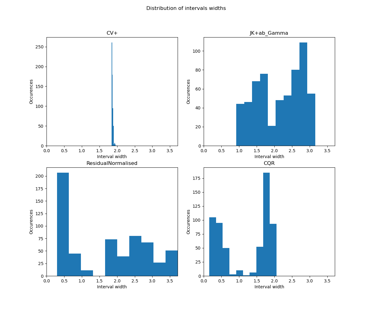
We would like to highlight here the misinterpretation that can be made with these metrics. In fact, here CV+ with the absolute residual score calculates constant intervals which, by definition, are not adaptive. Therefore, it is very important to check that the intervals widths are well spread before drawing conclusions (with a plot of the distribution of interval widths or a visualisation of the data for example).

In this example, with the hsic correlation coefficient, none of the methods stand out from the others. However, the SSC score for the method using the gamma score is significantly worse than for CQR and ResidualNormalisedScore, even though their global coverage is similar. ResidualNormalisedScore and CQR are very close here, with ResidualNormalisedScore being slightly more conservative.

# Visualition of the data and predictions
def plot_intervals(X, y, y_pred, intervals, title="", ax=None):
    """
    Plots the data X, y with associated intervals and predictions points.

    Parameters
    ----------
    X: ArrayLike
        Observed features
    y: ArrayLike
        Observed targets
    y_pred: ArrayLike
        Predictions
    intervals: ArrayLike
        Prediction intervals
    title: str
        Title of the plot
    ax: matplotlib axes
        An ax can be provided to include this plot in a subplot
    """
    if ax is None:
        fig, ax = plt.subplots(figsize=(6, 5))

    y_pred = y_pred.reshape((X.shape[0], 1))
    order = np.argsort(X[:, 0])

    # data
    ax.scatter(X.ravel(), y, color="#1f77b4", alpha=0.3, label="data")
    # predictions
    ax.scatter(
        X.ravel(), y_pred,
        color="#ff7f0e", marker="+", label="predictions", alpha=0.5
    )
    # intervals
    for i in range(intervals.shape[-1]):
        ax.fill_between(
            X[order].ravel(),
            intervals[:, 0, i][order],
            intervals[:, 1, i][order],
            color="#ff7f0e",
            alpha=0.3
        )

    ax.set_xlabel("x")
    ax.set_ylabel("y")
    ax.set_title(title)
    ax.legend()


def plot_coverage_by_width(y, intervals, num_bins, alpha, title="", ax=None):
    """
    PLots a bar diagram of coverages by groups of interval widths.

    Parameters
    ----------
    y: ArrayLike
        Observed targets.
    intervals: ArrayLike
        Intervals of prediction
    num_bins: int
        Number of groups of interval widths
    alpha: float
        The risk level
    title: str
        Title of the plot
    ax: matplotlib axes
        An ax can be provided to include this plot in a subplot
    """
    if ax is None:
        fig, ax = plt.subplots(figsize=(6, 5))

    ax.bar(
        np.arange(num_bins),
        regression_ssc(y, intervals, num_bins=num_bins)[0]
    )
    ax.axhline(y=1 - alpha, color='r', linestyle='-')
    ax.set_title(title)
    ax.set_xlabel("intervals grouped by size")
    ax.set_ylabel("coverage")
    ax.tick_params(
        axis='x', which='both', bottom=False, top=False, labelbottom=False
    )


max_width = np.max([
    np.abs(intervals[strategy][:, 0, 0] - intervals[strategy][:, 1, 0])
    for strategy in STRATEGIES.keys()])

fig_distr, axs_distr = plt.subplots(nrows=2, ncols=2, figsize=(12, 10))
fig_viz, axs_viz = plt.subplots(nrows=2, ncols=2, figsize=(12, 10))
fig_hist, axs_hist = plt.subplots(nrows=2, ncols=2, figsize=(12, 10))

for ax_viz, ax_hist, ax_distr, strategy in zip(
    axs_viz.flat, axs_hist.flat, axs_distr.flat, STRATEGIES.keys()
):
    plot_intervals(
        X_test, y_test, y_pred[strategy], intervals[strategy],
        title=strategy, ax=ax_viz
    )
    plot_coverage_by_width(
        y_test, intervals[strategy],
        num_bins=num_bins, alpha=alpha, title=strategy, ax=ax_hist
    )

    ax_distr.hist(
        np.abs(intervals[strategy][:, 0, 0] - intervals[strategy][:, 1, 0]),
        bins=num_bins
    )
    ax_distr.set_xlabel("Interval width")
    ax_distr.set_ylabel("Occurences")
    ax_distr.set_title(strategy)
    ax_distr.set_xlim([0, max_width])

fig_viz.suptitle("Predicted points and intervals on test data")
fig_distr.suptitle("Distribution of intervals widths")
fig_hist.suptitle("Coverage by bins of intervals grouped by widths (ssc)")
plt.tight_layout()
plt.show()

• 
• 
• 

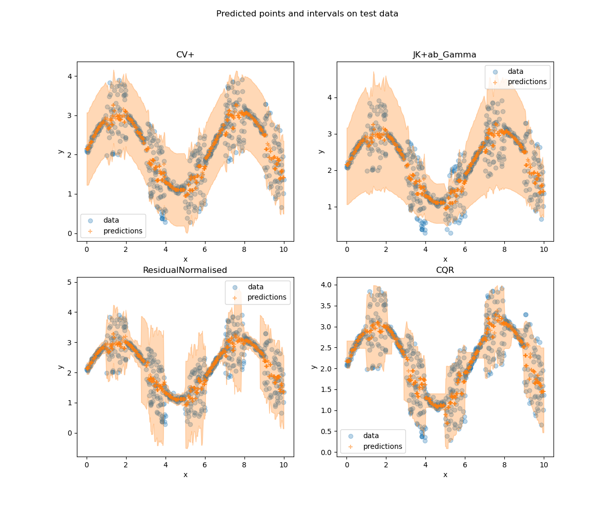
With toy datasets like this, it is easy to compare visually the methods with a plot of the data and predictions. As mentionned above, a histogram of the ditribution of the interval widths is important to accompany the metrics. It is clear from this histogram that CV+ is not adaptive, the metrics presented here should not be used to evaluate its adaptivity. A wider spread of intervals indicates a more adaptive method. 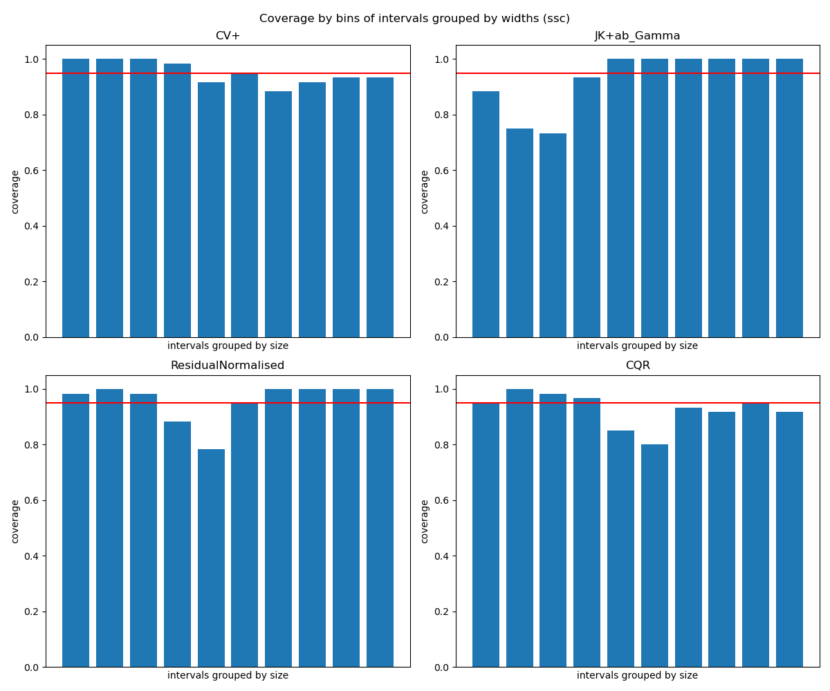Finally, with the plot of coverage by bins of intervals grouped by widths (which is the output of regression_ssc()), we want the bins to be as constant as possible around the global coverage (here 0.9).

# As the previous metrics show, gamma score does not perform well in terms of
# size stratified coverage. It either over-covers or under-covers too much.
# For ResidualNormalisedScore and CQR, while the first one has several bins
# with over-coverage, the second one has more under-coverage. These results
# are confirmed by the visualisation of the data: CQR is better when the data
# are more spread out, whereas ResidualNormalisedScore is better with small
# intervals.