Make Conformal Predictive Distribution with MAPIE

In this advanced analysis, we propose to use MAPIE for Conformal Predictive Distribution (CPD) in few steps. Here are some reference papers for more information about CPD:

[1] Schweder, T., & Hjort, N. L. (2016). Confidence, likelihood, probability (Vol. 41). Cambridge University Press.

[2] Vovk, V., Shen, J., Manokhin, V., & Xie, M. G. (2017, May). Nonparametric predictive distributions based on conformal prediction. In Conformal and probabilistic prediction and applications (pp. 82-102). PMLR.

import warnings

import numpy as np
from matplotlib import pyplot as plt
from sklearn.datasets import make_regression
from sklearn.linear_model import LinearRegression
from sklearn.model_selection import train_test_split

from mapie.conformity_scores import (AbsoluteConformityScore,
                                     ResidualNormalisedScore)
from mapie.regression import MapieRegressor

warnings.filterwarnings('ignore')

random_state = 15

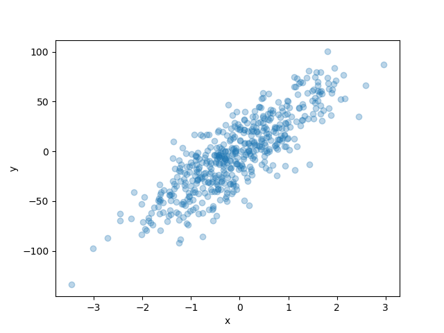
1. Generating toy dataset

Here, we propose just to generate data for regression task, then split it.

X, y = make_regression(
    n_samples=1000, n_features=1, noise=20, random_state=random_state
)
X_train, X_test, y_train, y_test = train_test_split(
    X, y, test_size=0.5, random_state=random_state
)

plt.xlabel("x")
plt.ylabel("y")
plt.scatter(X_train, y_train, alpha=0.3)
plt.show()

2. Defining a Conformal Predictive Distribution class with MAPIE

To be able to obtain the cumulative distribution function of a prediction with MAPIE, we propose here to wrap the MapieRegressor to add a new method named get_cumulative_distribution_function.

class MapieConformalPredictiveDistribution(MapieRegressor):

    def __init__(self, **kwargs) -> None:
        super().__init__(**kwargs)
        self.conformity_score.sym = False

    def get_cumulative_distribution_function(self, X):
        y_pred = self.predict(X)
        cs = self.conformity_scores_[~np.isnan(self.conformity_scores_)]
        res = self.conformity_score_function_.get_estimation_distribution(
            y_pred.reshape((-1, 1)), cs, X=X
        )
        return res

Now, we propose to use it with two different conformity scores - AbsoluteConformityScore and ResidualNormalisedScore - in split-conformal inference.

mapie_regressor_1 = MapieConformalPredictiveDistribution(
    estimator=LinearRegression(),
    conformity_score=AbsoluteConformityScore(),
    cv='split',
    random_state=random_state
)

mapie_regressor_1.fit(X_train, y_train)
y_pred_1 = mapie_regressor_1.predict(X_test)
y_cdf_1 = mapie_regressor_1.get_cumulative_distribution_function(X_test)

mapie_regressor_2 = MapieConformalPredictiveDistribution(
    estimator=LinearRegression(),
    conformity_score=ResidualNormalisedScore(),
    cv='split',
    random_state=random_state
)

mapie_regressor_2.fit(X_train, y_train)
y_pred_2 = mapie_regressor_2.predict(X_test)
y_cdf_2 = mapie_regressor_2.get_cumulative_distribution_function(X_test)

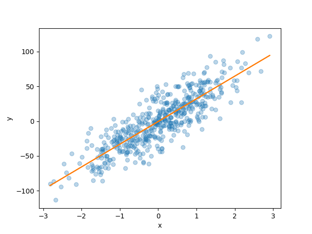
plt.xlabel("x")
plt.ylabel("y")
plt.scatter(X_test, y_test, alpha=0.3)
plt.plot(X_test, y_pred_1, color="C1")
plt.show()

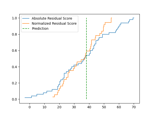
3. Visualizing the cumulative distribution function

We now propose to visualize the cumulative distribution functions of the predictive distribution in a graph in order to compare the two methods.

nb_bins = 100


def plot_cdf(data, bins, **kwargs):
    counts, bins = np.histogram(data, bins=bins)
    cdf = np.cumsum(counts)/np.sum(counts)

    plt.plot(
        np.vstack((bins, np.roll(bins, -1))).T.flatten()[:-2],
        np.vstack((cdf, cdf)).T.flatten(),
        **kwargs
    )


plot_cdf(
    y_cdf_1[0], bins=nb_bins, label='Absolute Residual Score', alpha=0.8
)
plot_cdf(
    y_cdf_2[0], bins=nb_bins, label='Normalized Residual Score', alpha=0.8
)
plt.vlines(
    y_pred_1[0], 0, 1, label='Prediction', color="C2", linestyles='dashed'
)
plt.legend(loc=2)
plt.show()