Estimating coverage width based criterion

This example uses MapieRegressor, MapieQuantileRegressor and metrics is used to estimate the coverage width based criterion of 1D homoscedastic data using different strategies. The coverage width based criterion is computed with the function coverage_width_based()

import os
import warnings

import matplotlib.pyplot as plt
import numpy as np
import pandas as pd
from sklearn.linear_model import LinearRegression, QuantileRegressor
from sklearn.pipeline import Pipeline
from sklearn.preprocessing import PolynomialFeatures

from mapie.metrics import (coverage_width_based, regression_coverage_score,
                           regression_mean_width_score)
from mapie.regression import MapieQuantileRegressor, MapieRegressor
from mapie.subsample import Subsample

os.environ["TF_CPP_MIN_LOG_LEVEL"] = "3"
warnings.filterwarnings("ignore")

Estimating the aleatoric uncertainty of heteroscedastic noisy data

Let’s define again the function and another simple function that generates one-dimensional data with normal noise uniformely in a given interval.

def x_sinx(x):
    """One-dimensional x*sin(x) function."""
    return x*np.sin(x)


def get_1d_data_with_heteroscedastic_noise(
    funct, min_x, max_x, n_samples, noise
):
    """
    Generate 1D noisy data uniformely from the given function
    and standard deviation for the noise.
    """
    np.random.seed(59)
    X_train = np.linspace(min_x, max_x, n_samples)
    np.random.shuffle(X_train)
    X_test = np.linspace(min_x, max_x, n_samples*5)
    y_train = (
        funct(X_train) +
        (np.random.normal(0, noise, len(X_train)) * X_train)
    )
    y_test = (
        funct(X_test) +
        (np.random.normal(0, noise, len(X_test)) * X_test)
    )
    y_mesh = funct(X_test)
    return (
        X_train.reshape(-1, 1), y_train, X_test.reshape(-1, 1), y_test, y_mesh
    )

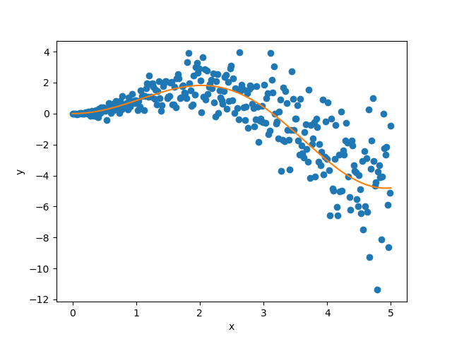
We first generate noisy one-dimensional data uniformely on an interval. Here, the noise is considered as heteroscedastic, since it will increase linearly with .

min_x, max_x, n_samples, noise = 0, 5, 300, 0.5
(
    X_train, y_train, X_test, y_test, y_mesh
) = get_1d_data_with_heteroscedastic_noise(
    x_sinx, min_x, max_x, n_samples, noise
)

Let’s visualize our noisy function. As x increases, the data becomes more noisy.

plt.xlabel("x")
plt.ylabel("y")
plt.scatter(X_train, y_train, color="C0")
plt.plot(X_test, y_mesh, color="C1")
plt.show()

As mentioned previously, we fit our training data with a simple polynomial function. Here, we choose a degree equal to 10 so the function is able to perfectly fit .

degree_polyn = 10
polyn_model = Pipeline(
    [
        ("poly", PolynomialFeatures(degree=degree_polyn)),
        ("linear", LinearRegression())
    ]
)
polyn_model_quant = Pipeline(
    [
        ("poly", PolynomialFeatures(degree=degree_polyn)),
        ("linear", QuantileRegressor(
                solver="highs",
                alpha=0,
        ))
    ]
)

We then estimate the prediction intervals for all the strategies very easily with a fit and predict process. The prediction interval’s lower and upper bounds are then saved in a DataFrame. Here, we set an alpha value of 0.05 in order to obtain a 95% confidence for our prediction intervals.

STRATEGIES = {
    "naive": dict(method="naive"),
    "jackknife": dict(method="base", cv=-1),
    "jackknife_plus": dict(method="plus", cv=-1),
    "jackknife_minmax": dict(method="minmax", cv=-1),
    "cv": dict(method="base", cv=10),
    "cv_plus": dict(method="plus", cv=10),
    "cv_minmax": dict(method="minmax", cv=10),
    "jackknife_plus_ab": dict(method="plus", cv=Subsample(n_resamplings=50)),
    "conformalized_quantile_regression": dict(
        method="quantile", cv="split", alpha=0.05
    )
}
y_pred, y_pis = {}, {}
for strategy, params in STRATEGIES.items():
    if strategy == "conformalized_quantile_regression":
        mapie = MapieQuantileRegressor(polyn_model_quant, **params)
        mapie.fit(X_train, y_train, random_state=1)
        y_pred[strategy], y_pis[strategy] = mapie.predict(X_test)
    else:
        mapie = MapieRegressor(polyn_model, **params)
        mapie.fit(X_train, y_train)
        y_pred[strategy], y_pis[strategy] = mapie.predict(X_test, alpha=0.05)

Once again, let’s compare the target confidence intervals with prediction intervals obtained with the Jackknife+, Jackknife-minmax, CV+, CV-minmax, Jackknife+-after-Boostrap, and CQR strategies.

def plot_1d_data(
    X_train,
    y_train,
    X_test,
    y_test,
    y_sigma,
    y_pred,
    y_pred_low,
    y_pred_up,
    ax=None,
    title=None
):
    ax.set_xlabel("x")
    ax.set_ylabel("y")
    ax.fill_between(X_test, y_pred_low, y_pred_up, alpha=0.3)
    ax.scatter(X_train, y_train, color="red", alpha=0.3, label="Training data")
    ax.plot(X_test, y_test, color="gray", label="True confidence intervals")
    ax.plot(X_test, y_test - y_sigma, color="gray", ls="--")
    ax.plot(X_test, y_test + y_sigma, color="gray", ls="--")
    ax.plot(
        X_test, y_pred, color="blue", alpha=0.5, label="Prediction intervals"
    )
    if title is not None:
        ax.set_title(title)
    ax.legend()


strategies = [
    "jackknife_plus",
    "jackknife_minmax",
    "cv_plus",
    "cv_minmax",
    "jackknife_plus_ab",
    "conformalized_quantile_regression"
]
n_figs = len(strategies)
fig, axs = plt.subplots(3, 2, figsize=(9, 13))
coords = [axs[0, 0], axs[0, 1], axs[1, 0], axs[1, 1], axs[2, 0], axs[2, 1]]
for strategy, coord in zip(strategies, coords):
    plot_1d_data(
        X_train.ravel(),
        y_train.ravel(),
        X_test.ravel(),
        y_mesh.ravel(),
        (1.96*noise*X_test).ravel(),
        y_pred[strategy].ravel(),
        y_pis[strategy][:, 0, 0].ravel(),
        y_pis[strategy][:, 1, 0].ravel(),
        ax=coord,
        title=strategy
    )
plt.show()

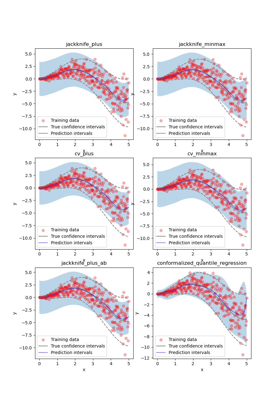
Let’s now conclude by summarizing the effective coverage, namely the fraction of test points whose true values lie within the prediction intervals, given by the different strategies.

coverage_score = {}
width_mean_score = {}
cwc_score = {}

for strategy in STRATEGIES:
    coverage_score[strategy] = regression_coverage_score(
        y_test,
        y_pis[strategy][:, 0, 0],
        y_pis[strategy][:, 1, 0]
    )
    width_mean_score[strategy] = regression_mean_width_score(
        y_pis[strategy][:, 0, 0],
        y_pis[strategy][:, 1, 0]
    )
    cwc_score[strategy] = coverage_width_based(
        y_test,
        y_pis[strategy][:, 0, 0],
        y_pis[strategy][:, 1, 0],
        eta=0.001,
        alpha=0.05
    )

results = pd.DataFrame(
    [
        [
            coverage_score[strategy],
            width_mean_score[strategy],
            cwc_score[strategy]
        ] for strategy in STRATEGIES
    ],
    index=STRATEGIES,
    columns=["Coverage", "Width average", "Coverage Width-based Criterion"]
).round(2)

print(results)

Out:

                                   Coverage  ...  Coverage Width-based Criterion
naive                                  0.94  ...                            0.61
jackknife                              0.95  ...                            0.59
jackknife_plus                         0.95  ...                            0.59
jackknife_minmax                       0.96  ...                            0.58
cv                                     0.95  ...                            0.60
cv_plus                                0.95  ...                            0.60
cv_minmax                              0.97  ...                            0.55
jackknife_plus_ab                      0.95  ...                            0.61
conformalized_quantile_regression      0.97  ...                            0.67

[9 rows x 3 columns]

All the strategies have the wanted coverage, however, we notice that the CQR strategy has much lower interval width than all the other methods, therefore, with heteroscedastic noise, CQR would be the preferred method.