Reproduction of part of the paper experiments of Zaffran et al. (2022)

MapieTimeSeriesRegressor is used to reproduce a part of the paper experiments of Zaffran et al. (2022) in their article [1] which we argue that Adaptive Conformal Inference (ACI, Gibbs & Candès, 2021) [2], developed for distribution-shift time series, is a good procedure for time series with general dependency.

For a given model, the simulation adjusts the MAPIE regressors using aci method, on a dataset taken from the article and available on the github repository https://github.com/mzaffran/AdaptiveConformalPredictionsTimeSeries and compares the bounds of the PIs.

In order to reproduce the results of the github repository, we reuse the RandomForestRegressor regression model and follow the same conformal prediction procedure (see in AdaptiveConformalPredictionsTimeSeries project the models.py file).

This simulation is carried out to check that the aci method implemented in MAPIE gives the same results as [1], and that the bounds of the PIs are obtained.

[1] Zaffran, M., Féron, O., Goude, Y., Josse, J., & Dieuleveut, A. (2022). Adaptive conformal predictions for time series. In International Conference on Machine Learning (pp. 25834-25866). PMLR.

[2] Gibbs, I., & Candes, E. (2021). Adaptive conformal inference under distribution shift. Advances in Neural Information Processing Systems, 34, 1660-1672.

import datetime
import pickle
import ssl
import warnings
from typing import Tuple
from urllib.request import urlopen

import numpy as np
import pandas as pd
from matplotlib import pylab as plt
from sklearn.ensemble import RandomForestRegressor
from sklearn.model_selection import PredefinedSplit

from mapie._typing import NDArray
from mapie.conformity_scores import AbsoluteConformityScore
from mapie.time_series_regression import MapieTimeSeriesRegressor

warnings.simplefilter("ignore")

Global random forests parameters

def init_model():
    # the number of trees in the forest
    n_estimators = 1000

    # the minimum number of samples required to be at a leaf node
    # (default skgarden's parameter)
    min_samples_leaf = 1

    # the number of features to consider when looking for the best split
    # (default skgarden's parameter)
    max_features = 6

    model = RandomForestRegressor(
        n_estimators=n_estimators,
        min_samples_leaf=min_samples_leaf,
        max_features=max_features,
        random_state=1,
    )

    return model

Get data

def get_data() -> pd.DataFrame:
    """
    Get the data from a CSV file containing prices from 2016 to 2019.

    Returns
    -------
    pd.DataFrame
        The DataFrame containing the price data.
    """
    website = "https://raw.githubusercontent.com/"
    page = "mzaffran/AdaptiveConformalPredictionsTimeSeries/"
    folder = "131656fe4c25251bad745f52db3c2d7cb1c24bbb/data_prices/"
    file = "Prices_2016_2019_extract.csv"
    url = website + page + folder + file
    ssl._create_default_https_context = ssl._create_unverified_context
    df = pd.read_csv(url)
    return df

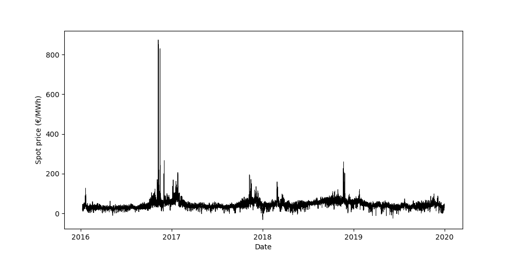
Get & Present data

data = get_data()

date_data = pd.to_datetime(data.Date)

plt.figure(figsize=(10, 5))
plt.plot(date_data, data.Spot, color="black", linewidth=0.6)

locs, labels = plt.xticks()
new_labels = ["2016", "2017", "2018", "2019", "2020"]
plt.xticks(locs[0:len(locs):2], labels=new_labels)

plt.xlabel("Date")
plt.ylabel("Spot price (\u20AC/MWh)")

plt.show()

Prepare data

limit = datetime.datetime(2019, 1, 1, tzinfo=datetime.timezone.utc)
id_train = data.index[pd.to_datetime(data['Date'], utc=True) < limit].tolist()

data_train = data.iloc[id_train, :]
sub_data_train = data_train.loc[:, [
    'hour', 'dow_0', 'dow_1', 'dow_2', 'dow_3', 'dow_4', 'dow_5', 'dow_6'
    ] + ['lag_24_%d' % i for i in range(24)] +
    ['lag_168_%d' % i for i in range(24)] + ['conso']
]
all_x_train = [
    np.array(sub_data_train.loc[sub_data_train.hour == h]) for h in range(24)
]

sub_data = data.loc[:, [
    'hour', 'dow_0', 'dow_1', 'dow_2', 'dow_3', 'dow_4', 'dow_5', 'dow_6'
    ] + ['lag_24_%d' % i for i in range(24)] +
    ['lag_168_%d' % i for i in range(24)] + ['conso']
]

all_x = [np.array(sub_data.loc[sub_data.hour == h]) for h in range(24)]
all_y = [np.array(data.loc[data.hour == h, 'Spot']) for h in range(24)]

Select Data (hour 0)

h = 0  # Let define hour = 0

X = all_x[h]
Y = all_y[h]

n = len(Y)
train_size = all_x_train[0].shape[0]
test_size = n - train_size

idx = np.array(range(train_size))
n_half = int(np.floor(train_size / 2))
idx_train, idx_cal = idx[:n_half], idx[n_half:2*n_half]

Prepare model

iteration_max = 10
alpha = 0.1
gamma = 0.04

model = init_model()

mapie_aci = MapieTimeSeriesRegressor(
    model,
    method="aci",
    agg_function="mean",
    conformity_score=AbsoluteConformityScore(sym=True),
    cv=PredefinedSplit(test_fold=[-1] * n_half + [0] * n_half),
    random_state=1,
)

Reproduce experiment and results

y_pred_aci_pfit = np.zeros(((365, )))
y_pis_aci_pfit = np.zeros(((365, 2, 1)))

for i in range(min(test_size, iteration_max + 1)):
    x_train = np.array(X[i:(train_size+i), ])
    x_test = np.array(X[(train_size+i), ]).reshape(1, -1)
    y_train = np.array(Y[i:(train_size+i)])
    y_test = np.array(Y[(train_size+i)]).reshape(1, -1)

    # Fit the model with new tran/calib dataset
    mapie_aci = mapie_aci.fit(x_train, y_train)

    # Predict on test dataset
    y_pred_aci_pfit[i:i+1], y_pis_aci_pfit[i:i+1] = mapie_aci.predict(
        x_test, alpha=alpha, ensemble=False, optimize_beta=False
    )

    # Update the current_alpha_t (hidden for the user)
    mapie_aci.update(
        x_test, y_test, gamma=gamma, ensemble=False, optimize_beta=False
    )

results = y_pis_aci_pfit.copy()

Get referenced result to reproduce

def get_pickle() -> Tuple[NDArray, NDArray]:
    """
    Get the pickle file containing the loaded data.

    Returns
    -------
    Tuple[NDArray, NDArray]
        A tuple containing the loaded data.
    """
    website = "https://github.com/"
    page = "mzaffran/AdaptiveConformalPredictionsTimeSeries/raw/"
    folder = "131656fe4c25251bad745f52db3c2d7cb1c24bbb/results/"
    folder += "Spot_France_Hour_0_train_2019-01-01/"
    file = "ACP_0.04_RF.pkl"
    url = website + page + folder + file
    ssl._create_default_https_context = ssl._create_unverified_context
    try:
        loaded_data = pickle.load(urlopen(url))
    except FileNotFoundError:
        print(f"The file {file} was not found.")
    except Exception as e:
        print(f"An error occurred: {e}")
    return loaded_data


data_ref = get_pickle()

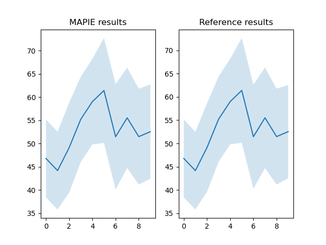
Compare results

# Flatten the array to shape (n, 2)
results_ref = np.concatenate([data_ref["Y_inf"], data_ref["Y_sup"]], axis=0).T
results = np.array(results.reshape(-1, 2))

# Compare the NumPy array with the corresponding DataFrame columns
comparison_result_Y_inf = np.allclose(
    results[:iteration_max, 0], results_ref[:iteration_max, 0], rtol=1e-2
)
comparison_result_Y_sup = np.allclose(
    results[:iteration_max, 1], results_ref[:iteration_max, 1], rtol=1e-2
)
comparison_result_Y_pred = np.allclose(
    y_pred_aci_pfit[:iteration_max], np.sum(results_ref, -1)[:iteration_max]/2,
    rtol=1e-2
)

# Print the comparison results
# The results are very closed but not exactly the same because of the quantile
# calculation. In MAPIE, we use method="higher" when in the code of Zaffran,
# it use method="midpoint".
final_results = pd.DataFrame({
    "y_inf": results[:iteration_max, 0],
    "y_inf (ref)": results_ref[:iteration_max, 0],
    "y_sup": results[:iteration_max, 1],
    "y_sup (ref)": results_ref[:iteration_max, 1],
    "y_pred": y_pred_aci_pfit[:iteration_max],
    "y_pred (ref)": np.sum(results_ref, -1)[:iteration_max]/2,
}).round(2)

idx = np.arange(iteration_max)
fig, axs = plt.subplots(1, 2)
axs[0].fill_between(
    idx, final_results["y_inf"], final_results["y_sup"],
    alpha=0.2
)
axs[0].plot(final_results["y_pred"])
axs[0].set_title("MAPIE results")
axs[1].fill_between(
    idx, final_results["y_inf (ref)"], final_results["y_sup (ref)"],
    alpha=0.2
)
axs[1].plot(final_results["y_pred (ref)"])
axs[1].set_title("Reference results")
plt.show()

print(final_results)
print(f"Comparison for ACP_0.04 (Y_inf): {comparison_result_Y_inf}")
print(f"Comparison for ACP_0.04 (Y_sup): {comparison_result_Y_sup}")
print(f"Comparison for ACP_0.04 (Y_pred): {comparison_result_Y_pred}")

Out:

   y_inf  y_inf (ref)  y_sup  y_sup (ref)  y_pred  y_pred (ref)
0  38.39        38.40  55.17        55.16   46.78         46.78
1  35.79        35.81  52.53        52.51   44.16         44.16
2  39.43        39.60  58.79        58.62   49.11         49.11
3  46.04        46.04  64.37        64.37   55.21         55.21
4  49.80        49.81  68.21        68.20   59.00         59.00
5  50.10        50.14  72.71        72.67   61.40         61.40
6  40.10        40.27  62.80        62.63   51.45         51.45
7  44.71        44.71  66.32        66.32   55.52         55.52
8  41.16        41.17  61.79        61.77   51.47         51.47
9  42.40        42.52  62.69        62.56   52.54         52.54
Comparison for ACP_0.04 (Y_inf): True
Comparison for ACP_0.04 (Y_sup): True
Comparison for ACP_0.04 (Y_pred): True