Estimating prediction intervals of Gamma distributed target

This example uses MapieRegressor to estimate prediction intervals associated with Gamma distributed target. The limit of the absolute residual conformity score is illustrated.

We use here the OpenML house_prices dataset: https://www.openml.org/search?type=data&sort=runs&id=42165&status=active.

The data is modelled by a Random Forest model RandomForestRegressor with a fixed parameter set. The prediction intervals are determined by means of the MAPIE regressor MapieRegressor considering two conformity scores: AbsoluteConformityScore which considers the absolute residuals as the conformity scores and GammaConformityScore which considers the residuals divided by the predicted means as conformity scores. We consider the standard CV+ resampling method.

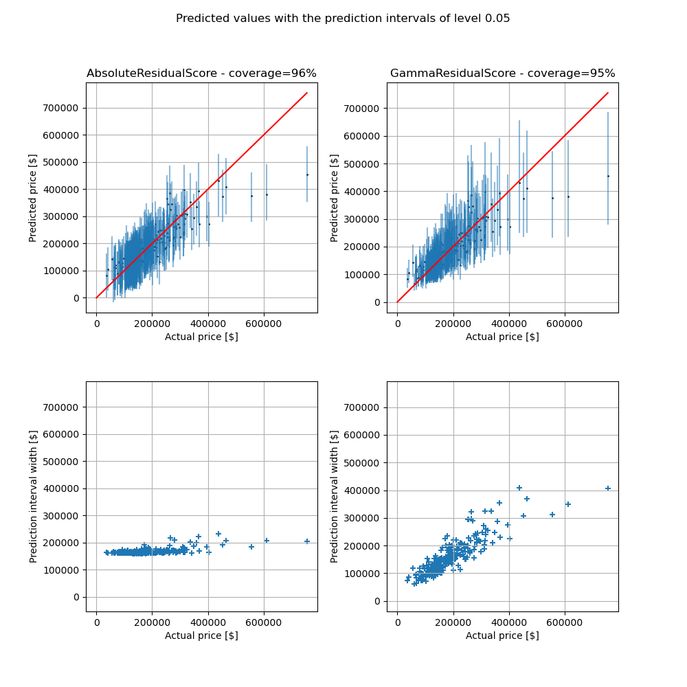
We would like to emphasize one main limitation with this example. With the default conformity score, the prediction intervals are approximately equal over the range of house prices which may be inapporpriate when the price range is wide. The Gamma conformity score overcomes this issue by considering prediction intervals with width proportional to the predicted mean. For low prices, the Gamma prediction intervals are narrower than the default ones, conversely to high prices for which the conficence intervals are higher but visually more relevant. The empirical coverage is similar between the two conformity scores.

import matplotlib.pyplot as plt
import numpy as np
from sklearn.datasets import fetch_openml
from sklearn.ensemble import RandomForestRegressor
from sklearn.model_selection import train_test_split

from mapie.conformity_scores import GammaConformityScore
from mapie.metrics import regression_coverage_score
from mapie.regression import MapieRegressor

random_state = 42

# Parameters
features = [
    "MSSubClass",
    "LotArea",
    "OverallQual",
    "OverallCond",
    "GarageArea",
]
alpha = 0.05
rf_kwargs = {"n_estimators": 10, "random_state": random_state}
model = RandomForestRegressor(**rf_kwargs)

1. Load dataset with a target following approximativeley a Gamma distribution

We start by loading a dataset with a target following approximately a Gamma distribution. The GammaConformityScore` is relevant in such cases. Two sub datasets are extracted: the training and test ones.

X, y = fetch_openml(name="house_prices", return_X_y=True)

X_train, X_test, y_train, y_test = train_test_split(
    X[features], y, test_size=0.2, random_state=random_state
)

Out:

/home/docs/checkouts/readthedocs.org/user_builds/mapie/conda/latest/lib/python3.10/site-packages/sklearn/datasets/_openml.py:1002: FutureWarning: The default value of `parser` will change from `'liac-arff'` to `'auto'` in 1.4. You can set `parser='auto'` to silence this warning. Therefore, an `ImportError` will be raised from 1.4 if the dataset is dense and pandas is not installed. Note that the pandas parser may return different data types. See the Notes Section in fetch_openml's API doc for details.
  warn(

2. Train model with two conformity scores

Two models are trained with two different conformity score:

• AbsoluteConformityScore (default conformity score) relevant for target positive as well as negative. The prediction interval widths are, in this case, approximately the same over the range of prediction.

• GammaConformityScore relevant for target following roughly a Gamma distribution. The prediction interval widths scale with the predicted value.

First, train model with AbsoluteConformityScore.

mapie = MapieRegressor(model, random_state=random_state)
mapie.fit(X_train, y_train)
y_pred_absconfscore, y_pis_absconfscore = mapie.predict(
    X_test, alpha=alpha, ensemble=True
)

coverage_absconfscore = regression_coverage_score(
    y_test, y_pis_absconfscore[:, 0, 0], y_pis_absconfscore[:, 1, 0]
)

Out:

/home/docs/checkouts/readthedocs.org/user_builds/mapie/conda/latest/lib/python3.10/site-packages/mapie/utils.py:598: UserWarning: WARNING: The predictions are ill-sorted.
  warnings.warn(

Prepare the results for matplotlib. Get the prediction intervals and their corresponding widths.

def get_yerr(y_pred, y_pis):
    return np.concatenate(
        [
            np.expand_dims(y_pred, 0) - y_pis[:, 0, 0].T,
            y_pis[:, 1, 0].T - np.expand_dims(y_pred, 0),
        ],
        axis=0,
    )


yerr_absconfscore = get_yerr(y_pred_absconfscore, y_pis_absconfscore)
pred_int_width_absconfscore = (
    y_pis_absconfscore[:, 1, 0] - y_pis_absconfscore[:, 0, 0]
)

Then, train the model with GammaConformityScore.

mapie = MapieRegressor(
    model, conformity_score=GammaConformityScore(), random_state=random_state
)
mapie.fit(X_train, y_train)
y_pred_gammaconfscore, y_pis_gammaconfscore = mapie.predict(
    X_test, alpha=[alpha], ensemble=True
)

coverage_gammaconfscore = regression_coverage_score(
    y_test, y_pis_gammaconfscore[:, 0, 0], y_pis_gammaconfscore[:, 1, 0]
)

yerr_gammaconfscore = get_yerr(y_pred_gammaconfscore, y_pis_gammaconfscore)
pred_int_width_gammaconfscore = (
    y_pis_gammaconfscore[:, 1, 0] - y_pis_gammaconfscore[:, 0, 0]
)

Out:

/home/docs/checkouts/readthedocs.org/user_builds/mapie/conda/latest/lib/python3.10/site-packages/mapie/utils.py:598: UserWarning: WARNING: The predictions are ill-sorted.
  warnings.warn(

3. Compare the prediction intervals

Once the models have been trained, we now compare the prediction intervals obtained from the two conformity scores. We can see that the AbsoluteConformityScore generates prediction interval with almost the same width for all the predicted values. Conversely, the mapie.conformity_scores.GammaConformityScore yields prediction interval with width scaling with the predicted values.

The choice of the conformity score depends on the problem we face.

fig, axs = plt.subplots(2, 2, figsize=(10, 10))

for img_id, y_pred, y_err, cov, class_name, int_width in zip(
    [0, 1],
    [y_pred_absconfscore, y_pred_gammaconfscore],
    [yerr_absconfscore, yerr_gammaconfscore],
    [coverage_absconfscore, coverage_gammaconfscore],
    ["AbsoluteResidualScore", "GammaResidualScore"],
    [pred_int_width_absconfscore, pred_int_width_gammaconfscore],
):
    axs[0, img_id].errorbar(
        y_test,
        y_pred,
        yerr=y_err,
        alpha=0.5,
        linestyle="None",
    )
    axs[0, img_id].scatter(y_test, y_pred, s=1, color="black")
    axs[0, img_id].plot(
        [0, max(max(y_test), max(y_pred))],
        [0, max(max(y_test), max(y_pred))],
        "-r",
    )
    axs[0, img_id].set_xlabel("Actual price [$]")
    axs[0, img_id].set_ylabel("Predicted price [$]")
    axs[0, img_id].grid()
    axs[0, img_id].set_title(f"{class_name} - coverage={cov:.0%}")

    xmin, xmax = axs[0, img_id].get_xlim()
    ymin, ymax = axs[0, img_id].get_ylim()
    axs[1, img_id].scatter(y_test, int_width, marker="+")
    axs[1, img_id].set_xlabel("Actual price [$]")
    axs[1, img_id].set_ylabel("Prediction interval width [$]")
    axs[1, img_id].grid()
    axs[1, img_id].set_xlim([xmin, xmax])
    axs[1, img_id].set_ylim([ymin, ymax])

fig.suptitle(
    f"Predicted values with the prediction intervals of level {alpha}"
)
plt.subplots_adjust(wspace=0.3, hspace=0.3)
plt.show()