Example use of the prefit parameter with neural networks and LGBM Regressor

MapieRegressor and MapieQuantileRegressor are used to calibrate uncertainties for large models for which the cost of cross-validation is too high. Typically, neural networks rely on a single validation set.

In this example, we first fit a neural network on the training set. We then compute residuals on a validation set with the cv=”prefit” parameter. Finally, we evaluate the model with prediction intervals on a testing set. We will also show how to use the prefit method in the conformalized quantile regressor.

import warnings

import numpy as np
import scipy
from lightgbm import LGBMRegressor
from matplotlib import pyplot as plt
from sklearn.model_selection import train_test_split
from sklearn.neural_network import MLPRegressor

from mapie._typing import NDArray
from mapie.metrics import regression_coverage_score
from mapie.regression import MapieQuantileRegressor, MapieRegressor

warnings.filterwarnings("ignore")

alpha = 0.1

1. Generate dataset

We start by defining a function that we will use to generate data. We then add random noise to the y values. Then we split the dataset to have a training, calibration and test set.

def f(x: NDArray) -> NDArray:
    """Polynomial function used to generate one-dimensional data."""
    return np.array(5 * x + 5 * x**4 - 9 * x**2)


# Generate data
sigma = 0.1
n_samples = 10000
X = np.linspace(0, 1, n_samples)
y = f(X) + np.random.normal(0, sigma, n_samples)

# Train/validation/test split
X_train_cal, X_test, y_train_cal, y_test = train_test_split(
    X, y, test_size=1 / 10
)
X_train, X_cal, y_train, y_cal = train_test_split(
    X_train_cal, y_train_cal, test_size=1 / 9
)

2. Pre-train models

For this example, we will train a MLPRegressor for MapieRegressor and multiple LGBMRegressor with a quantile objective as this is a requirement to perform conformalized quantile regression using MapieQuantileRegressor. Note that the three estimators need to be trained at quantile values of .

# Train a MLPRegressor for MapieRegressor
est_mlp = MLPRegressor(activation="relu", random_state=1)
est_mlp.fit(X_train.reshape(-1, 1), y_train)

# Train LGBMRegressor models for MapieQuantileRegressor
list_estimators_cqr = []
for alpha_ in [alpha / 2, (1 - (alpha / 2)), 0.5]:
    estimator_ = LGBMRegressor(
        objective='quantile',
        alpha=alpha_,
    )
    estimator_.fit(X_train.reshape(-1, 1), y_train)
    list_estimators_cqr.append(estimator_)

3. Using MAPIE to calibrate the models

We will now proceed to calibrate the models using MAPIE. To this aim, we set cv=”prefit” so that we use the models that we already trained prior. We then precict using the test set and evaluate its coverage.

# Calibrate uncertainties on calibration set
mapie = MapieRegressor(est_mlp, cv="prefit")
mapie.fit(X_cal.reshape(-1, 1), y_cal)

# Evaluate prediction and coverage level on testing set
y_pred, y_pis = mapie.predict(X_test.reshape(-1, 1), alpha=alpha)
coverage = regression_coverage_score(y_test, y_pis[:, 0, 0], y_pis[:, 1, 0])

# Calibrate uncertainties on calibration set
mapie_cqr = MapieQuantileRegressor(list_estimators_cqr, cv="prefit")
mapie_cqr.fit(X_cal.reshape(-1, 1), y_cal)

# Evaluate prediction and coverage level on testing set
y_pred_cqr, y_pis_cqr = mapie_cqr.predict(X_test.reshape(-1, 1))
coverage_cqr = regression_coverage_score(
    y_test,
    y_pis_cqr[:, 0, 0],
    y_pis_cqr[:, 1, 0]
)

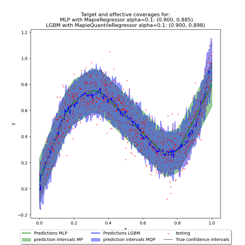
4. Plots

In order to view the results shown above, we will plot each other predictions with their prediction interval. The multi-layer perceptron (MLP) with MapieRegressor and LGBMRegressor with MapieQuantileRegressor.

# Plot obtained prediction intervals on testing set
theoretical_semi_width = scipy.stats.norm.ppf(1 - alpha) * sigma
y_test_theoretical = f(X_test)
order = np.argsort(X_test)

plt.figure(figsize=(8, 8))
plt.plot(
    X_test[order],
    y_pred[order],
    label="Predictions MLP",
    color="green"
)
plt.fill_between(
    X_test[order],
    y_pis[:, 0, 0][order],
    y_pis[:, 1, 0][order],
    alpha=0.4,
    label="prediction intervals MP",
    color="green"
)
plt.plot(
    X_test[order],
    y_pred_cqr[order],
    label="Predictions LGBM",
    color="blue"
)
plt.fill_between(
    X_test[order],
    y_pis_cqr[:, 0, 0][order],
    y_pis_cqr[:, 1, 0][order],
    alpha=0.4,
    label="prediction intervals MQP",
    color="blue"
)
plt.title(
    f"Target and effective coverages for:\n "
    f"MLP with MapieRegressor alpha={alpha}: "
    + f"({1 - alpha:.3f}, {coverage:.3f})\n"
    f"LGBM with MapieQuantileRegressor alpha={alpha}: "
    + f"({1 - alpha:.3f}, {coverage_cqr:.3f})"
)
plt.scatter(X_test, y_test, color="red", alpha=0.7, label="testing", s=2)
plt.plot(
    X_test[order],
    y_test_theoretical[order],
    color="gray",
    label="True confidence intervals",
)
plt.plot(
    X_test[order],
    y_test_theoretical[order] - theoretical_semi_width,
    color="gray",
    ls="--",
)
plt.plot(
    X_test[order],
    y_test_theoretical[order] + theoretical_semi_width,
    color="gray",
    ls="--",
)
plt.xlabel("x")
plt.ylabel("y")
plt.legend(
    loc='upper center',
    bbox_to_anchor=(0.5, -0.05),
    fancybox=True,
    shadow=True,
    ncol=3
)
plt.show()